

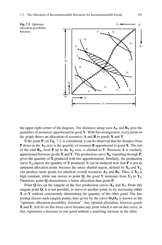
the upper right corner of the diagram. The distances along axes A Y and B Y give the
quantities of resources apportioned to good Y. With this arrangement, every point on
the graph shows an allocation of resources A and B to goods X and Y.
If the point P, on Fig. 7.2, is considered, it can be observed that the distance from
P down to the A X axis is the quantity of resource B apportioned to good X. The rest
of the total B T , from P up to the A Y axis, is allotted to Y. Resource A is similarly
apportioned between goods X and Y. The production curve X 2 , transiting through P,
gives the quantity of X produced with this apportionment. Similarly, the production
curve Y 2 depicts the quantity of Y produced. It can be deduced now that P is not an
optimum allocation point, because the entire shaded region, defined by X 2 and Y 2 ,
can produce more goods for identical overall resources A T and B T . Thus, if X 2 is
kept constant, while one moves to point Q, the good Y increases from Y 2 to Y 3 .
Therefore, point Q characterises a better allocation than point P.
Point Q lies on the tangent of the two production curves X 2 and Y 3 . From this
tangent point Q, it is not possible, to move to another point, to try increasing either
X or Y without concurrently diminishing the quantity of the other good. The line
joining (locus) such tangent points, here given by the curve O X O Y is known as the
“optimum allocation possibility function”. Any optimal allocation, between goods
X and Y, will lie on this locus curve because any point which is not on this curve, in
fact, represents a decrease in one good without a matching increase in the other.
X1
X2
X3
X2
X1
Y2
Y3
Y2
Y1
Y1
X3
Y3
Y4
AY
AX
OX
B X
B
P
Q
Y
A Y
B Y
O Y
Y4
Fig. 7.2 Optimum
allocation possibility
function
7.3 The Allocation of Incommensurable Resources for Incommensurable Goods
191
quantities of resources apportioned to good Y. With this arrangement, every point on
the graph shows an allocation of resources A and B to goods X and Y.
If the point P, on Fig. 7.2, is considered, it can be observed that the distance from
P down to the A X axis is the quantity of resource B apportioned to good X. The rest
of the total B T , from P up to the A Y axis, is allotted to Y. Resource A is similarly
apportioned between goods X and Y. The production curve X 2 , transiting through P,
gives the quantity of X produced with this apportionment. Similarly, the production
curve Y 2 depicts the quantity of Y produced. It can be deduced now that P is not an
optimum allocation point, because the entire shaded region, defined by X 2 and Y 2 ,
can produce more goods for identical overall resources A T and B T . Thus, if X 2 is
kept constant, while one moves to point Q, the good Y increases from Y 2 to Y 3 .
Therefore, point Q characterises a better allocation than point P.
Point Q lies on the tangent of the two production curves X 2 and Y 3 . From this
tangent point Q, it is not possible, to move to another point, to try increasing either
X or Y without concurrently diminishing the quantity of the other good. The line
joining (locus) such tangent points, here given by the curve O X O Y is known as the
“optimum allocation possibility function”. Any optimal allocation, between goods
X and Y, will lie on this locus curve because any point which is not on this curve, in
fact, represents a decrease in one good without a matching increase in the other.
X1
X2
X3
X2
X1
Y2
Y3
Y2
Y1
Y1
X3
Y3
Y4
AY
AX
OX
B X
B
P
Q
Y
A Y
B Y
O Y
Y4
Fig. 7.2 Optimum
allocation possibility
function
7.3 The Allocation of Incommensurable Resources for Incommensurable Goods
191