

Consider first the good X, where, following a given outlay of resources A and B, a
corresponding unique amount of good X is obtained. Furthermore, any increase in
the outlay of either A or B, will entail an increase in the quantity of good X, but, at
least, no reduction, in the worst case. Thus, one can plot, for a specified amount of
the good X, say X 1 , the relationship between the required outlays of A and of B
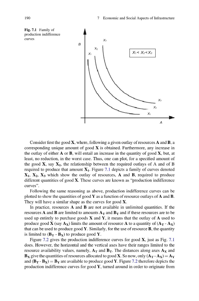
required to produce that amount X 1 . Figure 7.1 depicts a family of curves denoted
X 1 , X 2 , X 3 which show the outlay of resources, A and B, required to produce
different quantities of good X. These curves are known as “production indifference
curves”.
Following the same reasoning as above, production indifference curves can be
plotted to show the quantities of good Y as a function of resource outlays of A and B.
They will have a similar shape as the curves for good X.
In practice, resources A and B are not available in unlimited quantities. If the
resources A and B are limited to amounts A T and B T and if these resources are to be
used up entirely to purchase goods X and Y, it means that the outlay of A used to
produce good X (say A X ) limits the amount of resource A to a quantity of (A T - A X )
that can be used to produce good Y. Similarly, for the use of resource B, the quantity
is limited to (B T - B X ) to produce good Y.
Figure 7.2 gives the production indifference curves for good X, just as Fig. 7.1
does. However, the horizontal and the vertical axes have their ranges limited to the
resource availability values, namely, A T and B T . The distances along axes A X and
B X give the quantities of resources allocated to good X. So now, only (A T - A X ) ¼ A Y
and (B T - B X ) ¼ B Y are available to produce good Y. Figure 7.2 therefore depicts the
production indifference curves for good Y, turned around in order to originate from
A
B
X1 ˂ X2 ˂ X3
X3
X2
X1
X3
X1
X2
Fig. 7.1 Family of
production indifference
curves
190
7 Economic and Social Aspects of Infrastructure
corresponding unique amount of good X is obtained. Furthermore, any increase in
the outlay of either A or B, will entail an increase in the quantity of good X, but, at
least, no reduction, in the worst case. Thus, one can plot, for a specified amount of
the good X, say X 1 , the relationship between the required outlays of A and of B
required to produce that amount X 1 . Figure 7.1 depicts a family of curves denoted
X 1 , X 2 , X 3 which show the outlay of resources, A and B, required to produce
different quantities of good X. These curves are known as “production indifference
curves”.
Following the same reasoning as above, production indifference curves can be
plotted to show the quantities of good Y as a function of resource outlays of A and B.
They will have a similar shape as the curves for good X.
In practice, resources A and B are not available in unlimited quantities. If the
resources A and B are limited to amounts A T and B T and if these resources are to be
used up entirely to purchase goods X and Y, it means that the outlay of A used to
produce good X (say A X ) limits the amount of resource A to a quantity of (A T - A X )
that can be used to produce good Y. Similarly, for the use of resource B, the quantity
is limited to (B T - B X ) to produce good Y.
Figure 7.2 gives the production indifference curves for good X, just as Fig. 7.1
does. However, the horizontal and the vertical axes have their ranges limited to the
resource availability values, namely, A T and B T . The distances along axes A X and
B X give the quantities of resources allocated to good X. So now, only (A T - A X ) ¼ A Y
and (B T - B X ) ¼ B Y are available to produce good Y. Figure 7.2 therefore depicts the
production indifference curves for good Y, turned around in order to originate from
A
B
X1 ˂ X2 ˂ X3
X3
X2
X1
X3
X1
X2
Fig. 7.1 Family of
production indifference
curves
190
7 Economic and Social Aspects of Infrastructure