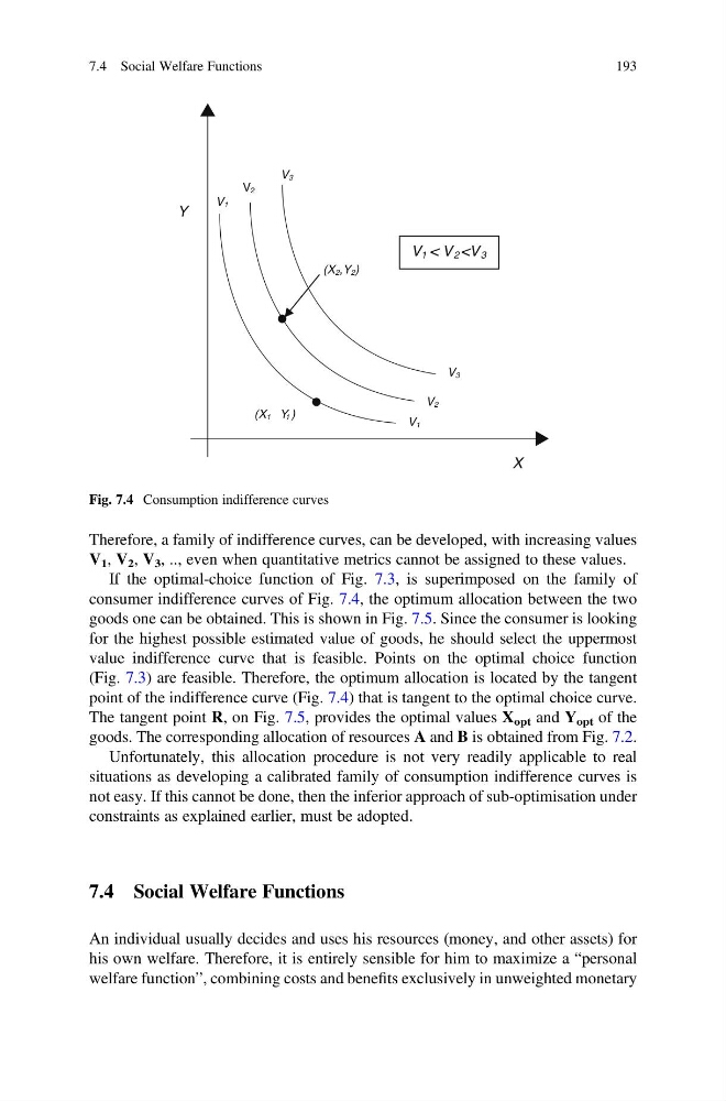
Therefore, a family of indifference curves, can be developed, with increasing values
V 1 , V 2 , V 3 , .., even when quantitative metrics cannot be assigned to these values.
If the optimal-choice function of Fig. 7.3, is superimposed on the family of
consumer indifference curves of Fig. 7.4, the optimum allocation between the two
goods one can be obtained. This is shown in Fig. 7.5. Since the consumer is looking
for the highest possible estimated value of goods, he should select the uppermost
value indifference curve that is feasible. Points on the optimal choice function
(Fig. 7.3) are feasible. Therefore, the optimum allocation is located by the tangent
point of the indifference curve (Fig. 7.4) that is tangent to the optimal choice curve.
The tangent point R, on Fig. 7.5, provides the optimal values X opt and Y opt of the
goods. The corresponding allocation of resources A and B is obtained from Fig. 7.2.
Unfortunately, this allocation procedure is not very readily applicable to real
situations as developing a calibrated family of consumption indifference curves is
not easy. If this cannot be done, then the inferior approach of sub-optimisation under
constraints as explained earlier, must be adopted.
7.4 Social Welfare Functions
An individual usually decides and uses his resources (money, and other assets) for
his own welfare. Therefore, it is entirely sensible for him to maximize a “personal
welfare function”, combining costs and benefits exclusively in unweighted monetary
V3
V2
V1
V < V 1
2
3
V3
V2
V1
X
Y
(X Y )
1
1
(X2,Y2)
Fig. 7.4 Consumption indifference curves
7.4 Social Welfare Functions
193