

excitation coefficients at variation of А ¼ α, while the coefficient В ¼ β ¼ const
remains unchanged.
Presented in Fig. 7.23 plots give us the possibility to select correctly the generation mode, tuning ranges, to estimate the linearity of adjusting functions of OEO
with the differential RF FODL. These calculated functions are true and interesting
for us at utilization in OEO of devices for variations of excitation coefficients А ¼ α,
В ¼ β on the base of electro-optical controlling elements (Fig. 7.24) or the modern
MZ modulators on LiNbO 3 .
Let us introduce, as in Eqs. (7.53) and (7.54), the following designations for the
difference between the delay time in light guides and for average delays in FOS:
T 1FOS ¼
T 2FOS þT 1FOS
2
À
T 2FOS ÀT 1FOS
2
, T 2FOS ¼
T 2FOS þT 1FOS
2
þ
T 2FOS ÀT 1FOS
2
.
Now we obtain equations for the frequency and the amplitude of the OEO
generation signal. At А ¼ В (i.e., at equal light power passed in channels), the
phase balance equation (7.50) can be transformed.
The approximate expression for the OEO generated frequency ω ¼ ω gen ¼ 2πf gen
can be derived from Eq. (7.50) and presented as: ω gen ffi (2πm + ω F T F )/
[0.5T 1FOS + 0.5T 2FOS + T L + T F ].
At the value A % B of approximately (but not exactly) equal of excitation
coefficients, we can derive the formula ω gen ffi 2πm + ω F T F ]/
[AT 1FOS + BT 2FOS + T L + T F ] for calculation of the OEO generation frequency.
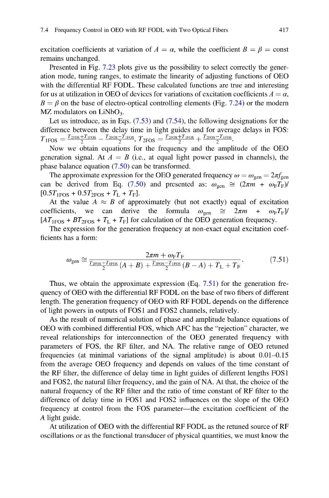
The expression for the generation frequency at non-exact equal excitation coefficients has a form:
ω gen ffi
2πm þ ω F T F
T 2FOS þT 1FOS
2
A þ B
ð
Þþ
T 2FOS ÀT 1FOS
2
B À A
ð
ÞþT L þ T F
:
ð7:51Þ
Thus, we obtain the approximate expression (Eq. 7.51) for the generation frequency of OEO with the differential RF FODL on the base of two fibers of different
length. The generation frequency of OEO with RF FODL depends on the difference
of light powers in outputs of FOS1 and FOS2 channels, relatively.
As the result of numerical solution of phase and amplitude balance equations of
OEO with combined differential FOS, which AFC has the “rejection” character, we
reveal relationships for interconnection of the OEO generated frequency with
parameters of FOS, the RF filter, and NA. The relative range of OEO retuned
frequencies (at minimal variations of the signal amplitude) is about 0.01–0.15
from the average OEO frequency and depends on values of the time constant of
the RF filter, the difference of delay time in light guides of different lengths FOS1
and FOS2, the natural filter frequency, and the gain of NA. At that, the choice of the
natural frequency of the RF filter and the ratio of time constant of RF filter to the
difference of delay time in FOS1 and FOS2 influences on the slope of the OEO
frequency at control from the FOS parameter—the excitation coefficient of the
A light guide.
At utilization of ОEO with the differential RF FODL as the retuned source of RF
oscillations or as the functional transducer of physical quantities, we must know the
7.4 Frequency Control in OEO with RF FODL with Two Optical Fibers
417
remains unchanged.
Presented in Fig. 7.23 plots give us the possibility to select correctly the generation mode, tuning ranges, to estimate the linearity of adjusting functions of OEO
with the differential RF FODL. These calculated functions are true and interesting
for us at utilization in OEO of devices for variations of excitation coefficients А ¼ α,
В ¼ β on the base of electro-optical controlling elements (Fig. 7.24) or the modern
MZ modulators on LiNbO 3 .
Let us introduce, as in Eqs. (7.53) and (7.54), the following designations for the
difference between the delay time in light guides and for average delays in FOS:
T 1FOS ¼
T 2FOS þT 1FOS
2
À
T 2FOS ÀT 1FOS
2
, T 2FOS ¼
T 2FOS þT 1FOS
2
þ
T 2FOS ÀT 1FOS
2
.
Now we obtain equations for the frequency and the amplitude of the OEO
generation signal. At А ¼ В (i.e., at equal light power passed in channels), the
phase balance equation (7.50) can be transformed.
The approximate expression for the OEO generated frequency ω ¼ ω gen ¼ 2πf gen
can be derived from Eq. (7.50) and presented as: ω gen ffi (2πm + ω F T F )/
[0.5T 1FOS + 0.5T 2FOS + T L + T F ].
At the value A % B of approximately (but not exactly) equal of excitation
coefficients, we can derive the formula ω gen ffi 2πm + ω F T F ]/
[AT 1FOS + BT 2FOS + T L + T F ] for calculation of the OEO generation frequency.
The expression for the generation frequency at non-exact equal excitation coefficients has a form:
ω gen ffi
2πm þ ω F T F
T 2FOS þT 1FOS
2
A þ B
ð
Þþ
T 2FOS ÀT 1FOS
2
B À A
ð
ÞþT L þ T F
:
ð7:51Þ
Thus, we obtain the approximate expression (Eq. 7.51) for the generation frequency of OEO with the differential RF FODL on the base of two fibers of different
length. The generation frequency of OEO with RF FODL depends on the difference
of light powers in outputs of FOS1 and FOS2 channels, relatively.
As the result of numerical solution of phase and amplitude balance equations of
OEO with combined differential FOS, which AFC has the “rejection” character, we
reveal relationships for interconnection of the OEO generated frequency with
parameters of FOS, the RF filter, and NA. The relative range of OEO retuned
frequencies (at minimal variations of the signal amplitude) is about 0.01–0.15
from the average OEO frequency and depends on values of the time constant of
the RF filter, the difference of delay time in light guides of different lengths FOS1
and FOS2, the natural filter frequency, and the gain of NA. At that, the choice of the
natural frequency of the RF filter and the ratio of time constant of RF filter to the
difference of delay time in FOS1 and FOS2 influences on the slope of the OEO
frequency at control from the FOS parameter—the excitation coefficient of the
A light guide.
At utilization of ОEO with the differential RF FODL as the retuned source of RF
oscillations or as the functional transducer of physical quantities, we must know the
7.4 Frequency Control in OEO with RF FODL with Two Optical Fibers
417