

in light guides (channels) to the time constant of the RF filter: (T 2FOS À T 1FOS )/T F ,
and (3) the excitation coefficients of FOS1 and FOS2: А and В ¼ 1 – А.
7.4.3 The Analysis of the Generation Frequency Control
in OEO with the Differential RF FODL in the Steady
State
Dependences of the signal frequency and the amplitude versus FOS parameters in
steady state can be obtained from the phase and amplitude balance equations in
Chap. 3. We assume that transfer functions for QWLD, FOS, PD, RF F, and NA
together with the nonlinear characteristic of AE in NA are known.
On the base of Eqs. (7.53) and (7.54), taking into consideration the performed
analysis, we obtain the approximated expressions for the frequency and the amplitude of the signal generated by OEO with the combined RF FODL and examine the
functions for the frequency and the amplitude of the generated signal by the solution
of the phase and amplitude balance equations.
Let us consider the steady-state equations of OEO with combined RF FODL,
which is constructed on the base of the differential FOS from two light guides of
different length (Fig. 7.33). From Eqs. (7.53) and (7.54), the conditions of the
amplitude and phase balance for OEO with the combined RF FODL follow.
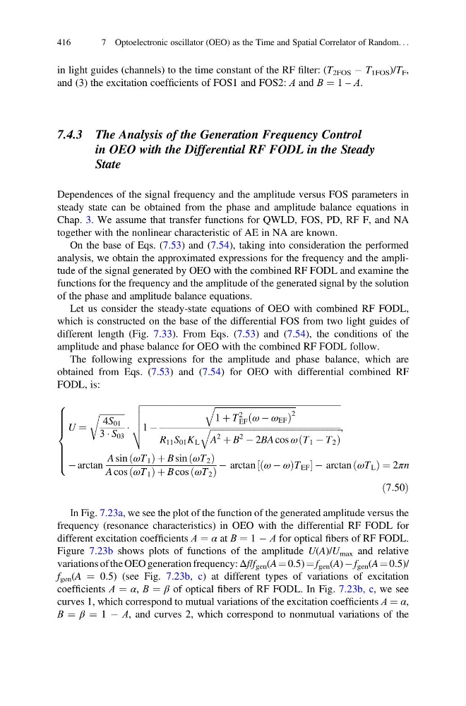
The following expressions for the amplitude and phase balance, which are
obtained from Eqs. (7.53) and (7.54) for OEO with differential combined RF
FODL, is:
U ¼
ffiffiffiffiffiffiffiffiffiffiffi ffi
4S 01
3 Á S 03
r
Á
ffiffiffiffiffiffiffiffiffiffiffiffiffiffiffiffiffiffiffiffiffiffiffiffiffiffiffiffiffiffiffiffiffiffiffiffiffiffiffiffiffiffiffiffiffiffiffiffiffiffiffiffiffiffiffiffiffiffiffiffiffiffiffiffiffiffiffiffiffiffiffiffiffiffiffiffiffiffiffiffiffiffiffiffiffiffiffiffiffiffi
1 À
ffiffiffiffiffiffiffiffiffiffiffiffiffiffiffiffiffiffiffiffiffiffiffiffiffiffiffiffiffiffiffiffiffiffiffiffiffi
1 þ T
2
EF ω À ω EF
ð
Þ
2
q
R 11 S 01 K L
ffiffiffiffiffiffiffiffiffiffiffiffiffiffiffiffiffiffiffiffiffiffiffiffiffiffiffiffiffiffiffiffiffiffiffiffiffiffiffiffiffiffiffiffiffiffiffiffiffiffiffiffiffiffiffiffiffiffiffi ffi
A
2
þ B
2
À 2BA cos ω T 1 À T 2
ð
Þ
q
v
u
u
u
t
,
À arctan
A sin ωT 1
ð
ÞþB sin ωT 2
ð
Þ
A cos ωT 1
ð
ÞþB cos ωT 2
ð
Þ
À arctan ω À ω
ð
ÞT EF
½
Àarctan ωT L
ð
Þ¼2πn
8
> > > > > <
> > > > > :
ð7:50Þ
In Fig. 7.23a, we see the plot of the function of the generated amplitude versus the
frequency (resonance characteristics) in OEO with the differential RF FODL for
different excitation coefficients А ¼ α at В ¼ 1 À А for optical fibers of RF FODL.
Figure 7.23b shows plots of functions of the amplitude U(A)/U max and relative
variations of the OEO generation frequency: Δf/f gen (A ¼ 0.5) ¼ f gen (A) À f gen (A ¼ 0.5)/
f gen (A ¼ 0.5) (see Fig. 7.23b, c) at different types of variations of excitation
coefficients А ¼ α, В ¼ β of optical fibers of RF FODL. In Fig. 7.23b, c, we see
curves 1, which correspond to mutual variations of the excitation coefficients А ¼ α,
В ¼ β ¼ 1 À А, and curves 2, which correspond to nonmutual variations of the
416
7 Optoelectronic oscillator (OEO) as the Time and Spatial Correlator of Random. . .
and (3) the excitation coefficients of FOS1 and FOS2: А and В ¼ 1 – А.
7.4.3 The Analysis of the Generation Frequency Control
in OEO with the Differential RF FODL in the Steady
State
Dependences of the signal frequency and the amplitude versus FOS parameters in
steady state can be obtained from the phase and amplitude balance equations in
Chap. 3. We assume that transfer functions for QWLD, FOS, PD, RF F, and NA
together with the nonlinear characteristic of AE in NA are known.
On the base of Eqs. (7.53) and (7.54), taking into consideration the performed
analysis, we obtain the approximated expressions for the frequency and the amplitude of the signal generated by OEO with the combined RF FODL and examine the
functions for the frequency and the amplitude of the generated signal by the solution
of the phase and amplitude balance equations.
Let us consider the steady-state equations of OEO with combined RF FODL,
which is constructed on the base of the differential FOS from two light guides of
different length (Fig. 7.33). From Eqs. (7.53) and (7.54), the conditions of the
amplitude and phase balance for OEO with the combined RF FODL follow.
The following expressions for the amplitude and phase balance, which are
obtained from Eqs. (7.53) and (7.54) for OEO with differential combined RF
FODL, is:
U ¼
ffiffiffiffiffiffiffiffiffiffiffi ffi
4S 01
3 Á S 03
r
Á
ffiffiffiffiffiffiffiffiffiffiffiffiffiffiffiffiffiffiffiffiffiffiffiffiffiffiffiffiffiffiffiffiffiffiffiffiffiffiffiffiffiffiffiffiffiffiffiffiffiffiffiffiffiffiffiffiffiffiffiffiffiffiffiffiffiffiffiffiffiffiffiffiffiffiffiffiffiffiffiffiffiffiffiffiffiffiffiffiffiffi
1 À
ffiffiffiffiffiffiffiffiffiffiffiffiffiffiffiffiffiffiffiffiffiffiffiffiffiffiffiffiffiffiffiffiffiffiffiffiffi
1 þ T
2
EF ω À ω EF
ð
Þ
2
q
R 11 S 01 K L
ffiffiffiffiffiffiffiffiffiffiffiffiffiffiffiffiffiffiffiffiffiffiffiffiffiffiffiffiffiffiffiffiffiffiffiffiffiffiffiffiffiffiffiffiffiffiffiffiffiffiffiffiffiffiffiffiffiffiffi ffi
A
2
þ B
2
À 2BA cos ω T 1 À T 2
ð
Þ
q
v
u
u
u
t
,
À arctan
A sin ωT 1
ð
ÞþB sin ωT 2
ð
Þ
A cos ωT 1
ð
ÞþB cos ωT 2
ð
Þ
À arctan ω À ω
ð
ÞT EF
½
Àarctan ωT L
ð
Þ¼2πn
8
> > > > > <
> > > > > :
ð7:50Þ
In Fig. 7.23a, we see the plot of the function of the generated amplitude versus the
frequency (resonance characteristics) in OEO with the differential RF FODL for
different excitation coefficients А ¼ α at В ¼ 1 À А for optical fibers of RF FODL.
Figure 7.23b shows plots of functions of the amplitude U(A)/U max and relative
variations of the OEO generation frequency: Δf/f gen (A ¼ 0.5) ¼ f gen (A) À f gen (A ¼ 0.5)/
f gen (A ¼ 0.5) (see Fig. 7.23b, c) at different types of variations of excitation
coefficients А ¼ α, В ¼ β of optical fibers of RF FODL. In Fig. 7.23b, c, we see
curves 1, which correspond to mutual variations of the excitation coefficients А ¼ α,
В ¼ β ¼ 1 À А, and curves 2, which correspond to nonmutual variations of the
416
7 Optoelectronic oscillator (OEO) as the Time and Spatial Correlator of Random. . .