

of PD near the optical frequency, and by the difference between optical frequencies.
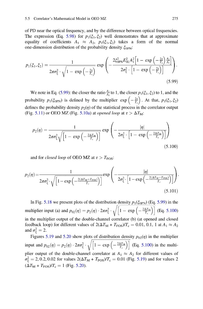
The expression (Eq. 5.98) for p 1 (ξ 1 , ξ 2 ) well demonstrates that at approximate
equality of coefficients A 1 % A 2 , p 1 (ξ 1 , ξ 2 ) takes a form of the normal
one-dimension distribution of the probability density ξ 0PN :
p 1 ξ 1 , ξ 2
ð
Þ¼
1
2πσ 2
ξ Á
ffiffiffiffiffiffiffiffiffiffiffiffiffiffiffiffiffiffiffiffiffiffiffiffiffiffiffiffiffiffi ffi
1 À exp À
2τ
T c
r
exp À
2ξ
2
0PN E
2
0L A
2
1 1 À exp À
2τ
T c
A 2
A 1
h
i
2σ 2
ξ Á 1 À exp À
2τ
T c
h
i
0
@
1
A :
ð5:99Þ
We note in Eq. (5.99): the closer the ratio
A 2
A 1
to 1, the closer p 1 (ξ 1 , ξ 2 ) to 1, and the
probability p 1 (ξ 0PN ) is defined by the multiplier exp À
2τ
T c
. At that, p 1 (ξ 1 , ξ 2 )
defines the probability density p 2 (η) of the statistical process in the correlator output
(Fig. 5.11) or OEO MZ (Fig. 5.10a) at opened loop at τ > ΔT M :
p 2 η
ð Þ ¼
1
2πσ 2
ξ
ffiffiffiffiffiffiffiffiffiffiffiffiffiffiffiffiffiffiffiffiffiffiffiffiffiffiffiffiffiffiffiffiffiffiffiffiffiffiffiffi ffi
1 À exp À
2ΔT M
T c
h
i
r
exp À
η
j j
2σ 2
ξ Á 1 À exp À
2ΔT M
T c
h
i
0
@
1
A
ð5:100Þ
and for closed loop of OEO MZ at τ > T FOS :
p 2 η
ð Þ¼
1
2πσ 2
ξ Á
ffiffiffiffiffiffiffiffiffiffiffiffiffiffiffiffiffiffiffiffiffiffiffiffiffiffiffiffiffiffiffiffiffiffiffiffiffiffiffiffiffiffiffiffiffiffiffiffiffi ffi
1À exp À
2 ΔT M þT FOS
ð
Þ
T c
h
i
r
exp À
η
j j
2σ 2
ξ Á 1À exp À
2 ΔT M þT FOS
ð
Þ
T c
h
i
0
@
1
A :
ð5:101Þ
In Fig. 5.18 we present plots of the distribution density p 1 (ξ 0PN ) (Eq. 5.99) in the
multiplier input (a) and p 02 η
ð Þ ¼ p 2 η
ð Þ Á 2πσ
2
ξ Á
ffiffiffiffiffiffiffiffiffiffiffiffiffiffiffiffiffiffiffiffiffiffiffiffiffiffiffiffiffiffiffiffiffiffiffiffiffiffiffiffi ffi
1 À exp À
2ΔT M
T c
h
i
r
(Eq. 5.100)
in the multiplier output of the double-channel correlator (b) (at opened and closed
feedback loop) for different values of 2(ΔT M + T FOS )/T c ¼ 0.01, 0.1, 1 at A 1 % A 2
and σ
2
ξ ¼ 2.
Figures 5.19 and 5.20 show plots of distribution density p 02 (η) in the multiplier
input and p 02 η
ð Þ ¼ p 2 η
ð Þ Á 2πσ
2
ξ Á
ffiffiffiffiffiffiffiffiffiffiffiffiffiffiffiffiffiffiffiffiffiffiffiffiffiffiffiffiffiffiffiffiffiffiffiffiffiffiffiffi ffi
1 À exp À
2ΔT M
T c
h
i
r
(Eq. 5.100) in the multiplier output of the double-channel correlator at A 1 % A 2 for different values of
σ
2
ξ ¼ 2, 0:2, 0:02 for values 2(ΔT M + T FOS )/T c ¼ 0.01 (Fig. 5.19) and for values 2
(ΔT M + T FOS )/T c ¼ 1 (Fig. 5.20).
5.5 Correlator’s Mathematical Model in OEO MZ
275
The expression (Eq. 5.98) for p 1 (ξ 1 , ξ 2 ) well demonstrates that at approximate
equality of coefficients A 1 % A 2 , p 1 (ξ 1 , ξ 2 ) takes a form of the normal
one-dimension distribution of the probability density ξ 0PN :
p 1 ξ 1 , ξ 2
ð
Þ¼
1
2πσ 2
ξ Á
ffiffiffiffiffiffiffiffiffiffiffiffiffiffiffiffiffiffiffiffiffiffiffiffiffiffiffiffiffiffi ffi
1 À exp À
2τ
T c
r
exp À
2ξ
2
0PN E
2
0L A
2
1 1 À exp À
2τ
T c
A 2
A 1
h
i
2σ 2
ξ Á 1 À exp À
2τ
T c
h
i
0
@
1
A :
ð5:99Þ
We note in Eq. (5.99): the closer the ratio
A 2
A 1
to 1, the closer p 1 (ξ 1 , ξ 2 ) to 1, and the
probability p 1 (ξ 0PN ) is defined by the multiplier exp À
2τ
T c
. At that, p 1 (ξ 1 , ξ 2 )
defines the probability density p 2 (η) of the statistical process in the correlator output
(Fig. 5.11) or OEO MZ (Fig. 5.10a) at opened loop at τ > ΔT M :
p 2 η
ð Þ ¼
1
2πσ 2
ξ
ffiffiffiffiffiffiffiffiffiffiffiffiffiffiffiffiffiffiffiffiffiffiffiffiffiffiffiffiffiffiffiffiffiffiffiffiffiffiffiffi ffi
1 À exp À
2ΔT M
T c
h
i
r
exp À
η
j j
2σ 2
ξ Á 1 À exp À
2ΔT M
T c
h
i
0
@
1
A
ð5:100Þ
and for closed loop of OEO MZ at τ > T FOS :
p 2 η
ð Þ¼
1
2πσ 2
ξ Á
ffiffiffiffiffiffiffiffiffiffiffiffiffiffiffiffiffiffiffiffiffiffiffiffiffiffiffiffiffiffiffiffiffiffiffiffiffiffiffiffiffiffiffiffiffiffiffiffiffi ffi
1À exp À
2 ΔT M þT FOS
ð
Þ
T c
h
i
r
exp À
η
j j
2σ 2
ξ Á 1À exp À
2 ΔT M þT FOS
ð
Þ
T c
h
i
0
@
1
A :
ð5:101Þ
In Fig. 5.18 we present plots of the distribution density p 1 (ξ 0PN ) (Eq. 5.99) in the
multiplier input (a) and p 02 η
ð Þ ¼ p 2 η
ð Þ Á 2πσ
2
ξ Á
ffiffiffiffiffiffiffiffiffiffiffiffiffiffiffiffiffiffiffiffiffiffiffiffiffiffiffiffiffiffiffiffiffiffiffiffiffiffiffiffi ffi
1 À exp À
2ΔT M
T c
h
i
r
(Eq. 5.100)
in the multiplier output of the double-channel correlator (b) (at opened and closed
feedback loop) for different values of 2(ΔT M + T FOS )/T c ¼ 0.01, 0.1, 1 at A 1 % A 2
and σ
2
ξ ¼ 2.
Figures 5.19 and 5.20 show plots of distribution density p 02 (η) in the multiplier
input and p 02 η
ð Þ ¼ p 2 η
ð Þ Á 2πσ
2
ξ Á
ffiffiffiffiffiffiffiffiffiffiffiffiffiffiffiffiffiffiffiffiffiffiffiffiffiffiffiffiffiffiffiffiffiffiffiffiffiffiffiffi ffi
1 À exp À
2ΔT M
T c
h
i
r
(Eq. 5.100) in the multiplier output of the double-channel correlator at A 1 % A 2 for different values of
σ
2
ξ ¼ 2, 0:2, 0:02 for values 2(ΔT M + T FOS )/T c ¼ 0.01 (Fig. 5.19) and for values 2
(ΔT M + T FOS )/T c ¼ 1 (Fig. 5.20).
5.5 Correlator’s Mathematical Model in OEO MZ
275