

T 1n G 00 , while Fig. 4.28 shows the QWLD resonance characteristics with the quadratic-hyperbolic nonlinearity at variation of the right part of Eq. (4.73) at saving of
the left part unchanged. In Fig. 4.28a at solution of Eq. (4.73) for values
T 1n G 00 ¼ 0.0001, the right part of (4.79) has the form S E 10n ¼ x
ð
Þ¼s
2
K 00 N 0 Áx
1þT 1n G 00 x
ð Þ
2 .
Figure 4.27 shows plots of the QWLD resonance characteristics with: quadratichyperbolic nonlinearity S E 10n
ð
Þ ¼
E 10n
ð
Þ
2 K 00 N 0
1þT 1n G 00 E
2
10n
for the second-order differential equation for Q 0F ¼ 0.4975: at quadratic-hyperbolic parametric dependence of the Qfactor: Q 0F ¼ 1/[2.01 À A Á (E 10n )
3 ], where A is the small parameter A ¼ 10
À9 .
From plots presented in Fig. 4.27 we can conclude that at the quadratic
nonlinearity S(E 10n ) at extremely small influence on Q 0F of the amplitude E 10n ,
QWLD at A ¼ 10
À9 transfers into the mode of chaotic oscillations, and its resonance
characteristic having regular branches at A ¼ 10
À10 (Fig. 4.27c) is completely
destroyed at A ¼ 10
À9 (Fig. 4.27d).
From an analysis of plots in Figs. 4.27 and 4.28 with the quadratic-hyperbolic
nonlinearity, we can make a conclusion that the laser exits on the mode of the steadystate generation only in the rigid self-excitation mode. These functions E 10n (ν/ν 0F )
differ qualitatively from the function at the linear-hyperbolic nonlinearity. In the plot
40
150
60
40
20
0
-20
-40
-60
100
50
2
1
2
3
2
1
1
0
2
1
20
0
-20
amplitude
x =
E
10n (s =
v /
v
0F ) (u.a.)
amplitude
x =
E
10n (s =
v /
v
0F ) (u.a.)
amplitude
x =
E
10n (s =
v /
v
0F ) (u.a.)
-40
-1.0 0.0
normalized optical
frequency
s = (v / v 0F ) (u.a.)
1.0
a)
-6 -2 0 2 4 6
normalized optical
frequency
s = (v / v 0F ) (u.a.)
b)
0.0 0.4
normalized optical
frequency
s = (v / v 0F ) (u.a.)
0.8
c)
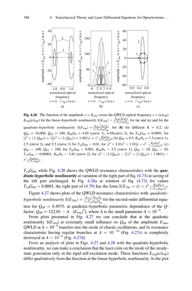
Fig. 4.26 The function of the amplitude x ¼ E 10n versus the QWLD optical frequency s ¼ (ν/ν 0F )
E 10n (ν/ν 0F ) for the linear-hyperbolic nonlinearity S E 10n
ð
Þ¼
E10n
ð
ÞK00N0
1þT1nG00E
2
10n
for (a) and (c) and for the
quadratic-hyperbolic nonlinearity S E 10n
ð
Þ¼
E10n
ð
Þ
2 K00N0
1þT1nG00E
2
10n
for (b) for different K ¼ 0.2: (а)
Q 0F ¼ 10,000, Q 02 ¼ 100, K 00 N 0 ¼ 4.05 (curve 1), 4.45(curve 2), for T 1n G 00 ¼ 0.0001, for
s
2 þ 1=Q 0F
ð
Þ s þ 1
½
s
2 þ 1=Q 02
ð
Þs þ 1:001
½
x ¼ s
1 K00N0x
1þT1nG00x 2 ; (b) Q 0F ¼ 0.5, K 00 N 0 ¼ 1.5 (curve 1),
2.5 (curve 2), and 5.5 (curve 3) for T 1n G 00 ¼ 0.01, for s
4 þ 2:01s
2 þ 1:01
½
x ¼ s
2 Á
K00N0x
2
1þT1nG00x 2 ; (с)
Q 0F ¼ 100, Q 02 ¼ 100, for T 1n G 00 ¼ 0.001, K 00 N 0 ¼ 3.5 (curve 1); Q 0F ¼ 10, Q 02 ¼ 10,
T 1n G 00 ¼ 0.00001, K 00 N 0 ¼ 3.45 (curve 2), for s
2 þ 1=Q 0F
ð
Þs þ 1
½
s
2 þ 1=Q 02
ð
Þs þ 1:001
½
x ¼
s
1 K00N0x
1þT1nG00x 2
186
4 Semiclassical Theory and Laser Differential Equations for Optoelectronic. . .
the left part unchanged. In Fig. 4.28a at solution of Eq. (4.73) for values
T 1n G 00 ¼ 0.0001, the right part of (4.79) has the form S E 10n ¼ x
ð
Þ¼s
2
K 00 N 0 Áx
1þT 1n G 00 x
ð Þ
2 .
Figure 4.27 shows plots of the QWLD resonance characteristics with: quadratichyperbolic nonlinearity S E 10n
ð
Þ ¼
E 10n
ð
Þ
2 K 00 N 0
1þT 1n G 00 E
2
10n
for the second-order differential equation for Q 0F ¼ 0.4975: at quadratic-hyperbolic parametric dependence of the Qfactor: Q 0F ¼ 1/[2.01 À A Á (E 10n )
3 ], where A is the small parameter A ¼ 10
À9 .
From plots presented in Fig. 4.27 we can conclude that at the quadratic
nonlinearity S(E 10n ) at extremely small influence on Q 0F of the amplitude E 10n ,
QWLD at A ¼ 10
À9 transfers into the mode of chaotic oscillations, and its resonance
characteristic having regular branches at A ¼ 10
À10 (Fig. 4.27c) is completely
destroyed at A ¼ 10
À9 (Fig. 4.27d).
From an analysis of plots in Figs. 4.27 and 4.28 with the quadratic-hyperbolic
nonlinearity, we can make a conclusion that the laser exits on the mode of the steadystate generation only in the rigid self-excitation mode. These functions E 10n (ν/ν 0F )
differ qualitatively from the function at the linear-hyperbolic nonlinearity. In the plot
40
150
60
40
20
0
-20
-40
-60
100
50
2
1
2
3
2
1
1
0
2
1
20
0
-20
amplitude
x =
E
10n (s =
v /
v
0F ) (u.a.)
amplitude
x =
E
10n (s =
v /
v
0F ) (u.a.)
amplitude
x =
E
10n (s =
v /
v
0F ) (u.a.)
-40
-1.0 0.0
normalized optical
frequency
s = (v / v 0F ) (u.a.)
1.0
a)
-6 -2 0 2 4 6
normalized optical
frequency
s = (v / v 0F ) (u.a.)
b)
0.0 0.4
normalized optical
frequency
s = (v / v 0F ) (u.a.)
0.8
c)
Fig. 4.26 The function of the amplitude x ¼ E 10n versus the QWLD optical frequency s ¼ (ν/ν 0F )
E 10n (ν/ν 0F ) for the linear-hyperbolic nonlinearity S E 10n
ð
Þ¼
E10n
ð
ÞK00N0
1þT1nG00E
2
10n
for (a) and (c) and for the
quadratic-hyperbolic nonlinearity S E 10n
ð
Þ¼
E10n
ð
Þ
2 K00N0
1þT1nG00E
2
10n
for (b) for different K ¼ 0.2: (а)
Q 0F ¼ 10,000, Q 02 ¼ 100, K 00 N 0 ¼ 4.05 (curve 1), 4.45(curve 2), for T 1n G 00 ¼ 0.0001, for
s
2 þ 1=Q 0F
ð
Þ s þ 1
½
s
2 þ 1=Q 02
ð
Þs þ 1:001
½
x ¼ s
1 K00N0x
1þT1nG00x 2 ; (b) Q 0F ¼ 0.5, K 00 N 0 ¼ 1.5 (curve 1),
2.5 (curve 2), and 5.5 (curve 3) for T 1n G 00 ¼ 0.01, for s
4 þ 2:01s
2 þ 1:01
½
x ¼ s
2 Á
K00N0x
2
1þT1nG00x 2 ; (с)
Q 0F ¼ 100, Q 02 ¼ 100, for T 1n G 00 ¼ 0.001, K 00 N 0 ¼ 3.5 (curve 1); Q 0F ¼ 10, Q 02 ¼ 10,
T 1n G 00 ¼ 0.00001, K 00 N 0 ¼ 3.45 (curve 2), for s
2 þ 1=Q 0F
ð
Þs þ 1
½
s
2 þ 1=Q 02
ð
Þs þ 1:001
½
x ¼
s
1 K00N0x
1þT1nG00x 2
186
4 Semiclassical Theory and Laser Differential Equations for Optoelectronic. . .