

n L ¼
T 1 α N0 À T 1 G 00 N 00 E n0 e L
j T 1 ν À ν 0F
ð
Þ=ν 0F
½
þ 1 þ T 1 G 00 E n0
ð Þ
2
:
ð4:64Þ
The operator control function in the small-signal mode can be defined as:
K L p 00
ð Þ ¼
K L00 p
2
00
p 4
00 þ а 10 p
3
00 þ а 20 À K 00 N 00
ð
Þ p 2
00 þ а 30 p 00 þ 1
ð4:65Þ
or in normalized frequency notation:
K L j ν=ν 0F
ð
Þ
½
¼
K L00 Á ν=ν 0F
ð
Þ
2
ν=ν 0F
ð
Þ
4 À jа 10 ν=ν 0F
ð
Þ
3 À а 20 À K 00 N 00
ð
Þν=ν 0F
ð
Þ
2 þ jа 30 ν=ν 0F
ð
Þþ1
,
ð4:66Þ
where
K L00 ¼
K 00 T 1 G 00 N 00 E 10n
j T 1 ν À ν 0F
ð
Þ=ν 0F
½
þ 1 þ T 1 G 00 Á E 10n
ð
Þ
2
:
ð4:67Þ
If ν % ν 0F in Eq. (4.67), K L00 ¼
K 00 T 1 G 00 N 00 E 10n
1þT 1 G 00 E 10n
ð
Þ
2 , K 00 ¼
2d
2
e
3Áε 0 2πh . In Eq. (4.66)
а 10 ¼ а 30 ¼
1
Q 0F
þ
1
Q 02
; а 20 % 2 þ
1
Q 0F Q 02
, а 20 % 2, а 10 % а 30 and depend on the
total losses in the system. Their values are varied from 0.008 to 0.0004 for different
types of lasers.
Figure 4.18 shows the poles diagram of the laser operator control function in the
state of the thermal equilibrium at the population difference less than (a) and higher
than (b) of the threshold value, at different Q-factors of the optical resonator and the
spectral line.
The plots of the module and argument of the operator control function for three
types of lasers (1—without quantum wells, 2—QWLD with the low resonator Q10
2
1
0.10
0.01
10
20
30
a)
b)
40
50
[1–
[2+
S’(E 10n )K 00 N 00
S’(E 10n )K 00 N 00
]
]
1
1
+
Q 0F
10
2
1
0.500
0.100
0.050
0.010
0.005
20
30
40
50
Q 0F
Q 02 = 10
Q 0F Q 02
Q 0F Q 02
v 12
2
v 0n
2
[1–
]
1
+ Q 0F Q 02
v 12
2
v 0n
2
[2+
]
1
Q 0F Q 02
Q 02 = 100
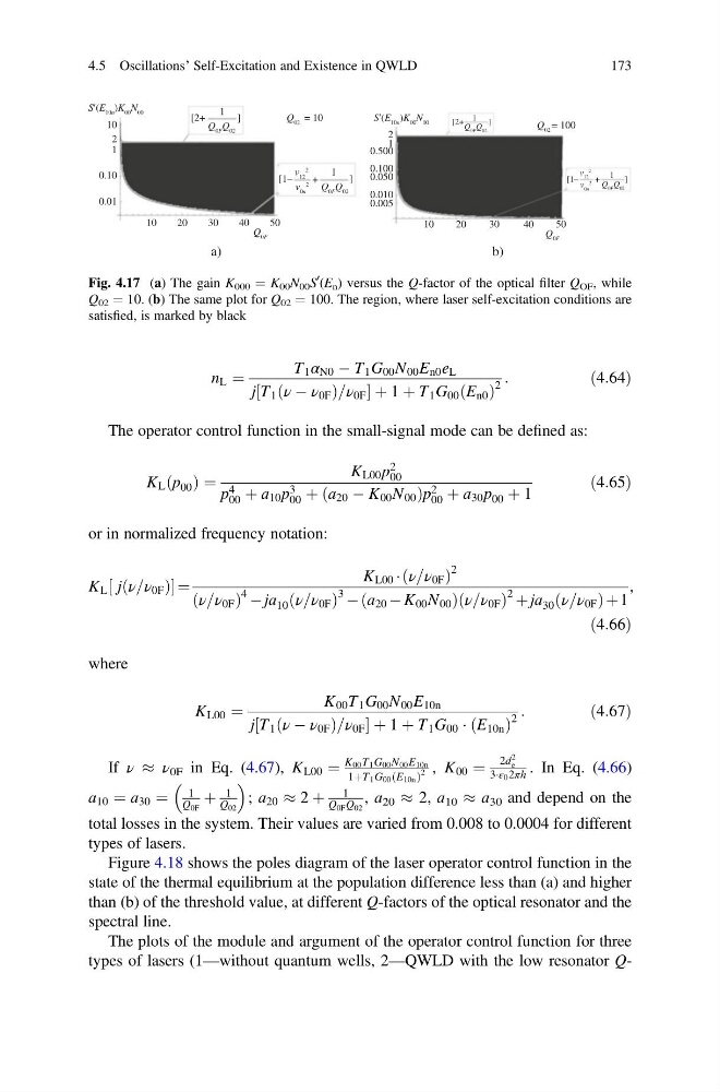
Fig. 4.17 (a) The gain K 000 ¼ K 00 N 00 S
0 (E n ) versus the Q-factor of the optical filter Q OF , while
Q 02 ¼ 10. (b) The same plot for Q 02 ¼ 100. The region, where laser self-excitation conditions are
satisfied, is marked by black
4.5 Oscillations’ Self-Excitation and Existence in QWLD
173
T 1 α N0 À T 1 G 00 N 00 E n0 e L
j T 1 ν À ν 0F
ð
Þ=ν 0F
½
þ 1 þ T 1 G 00 E n0
ð Þ
2
:
ð4:64Þ
The operator control function in the small-signal mode can be defined as:
K L p 00
ð Þ ¼
K L00 p
2
00
p 4
00 þ а 10 p
3
00 þ а 20 À K 00 N 00
ð
Þ p 2
00 þ а 30 p 00 þ 1
ð4:65Þ
or in normalized frequency notation:
K L j ν=ν 0F
ð
Þ
½
¼
K L00 Á ν=ν 0F
ð
Þ
2
ν=ν 0F
ð
Þ
4 À jа 10 ν=ν 0F
ð
Þ
3 À а 20 À K 00 N 00
ð
Þν=ν 0F
ð
Þ
2 þ jа 30 ν=ν 0F
ð
Þþ1
,
ð4:66Þ
where
K L00 ¼
K 00 T 1 G 00 N 00 E 10n
j T 1 ν À ν 0F
ð
Þ=ν 0F
½
þ 1 þ T 1 G 00 Á E 10n
ð
Þ
2
:
ð4:67Þ
If ν % ν 0F in Eq. (4.67), K L00 ¼
K 00 T 1 G 00 N 00 E 10n
1þT 1 G 00 E 10n
ð
Þ
2 , K 00 ¼
2d
2
e
3Áε 0 2πh . In Eq. (4.66)
а 10 ¼ а 30 ¼
1
Q 0F
þ
1
Q 02
; а 20 % 2 þ
1
Q 0F Q 02
, а 20 % 2, а 10 % а 30 and depend on the
total losses in the system. Their values are varied from 0.008 to 0.0004 for different
types of lasers.
Figure 4.18 shows the poles diagram of the laser operator control function in the
state of the thermal equilibrium at the population difference less than (a) and higher
than (b) of the threshold value, at different Q-factors of the optical resonator and the
spectral line.
The plots of the module and argument of the operator control function for three
types of lasers (1—without quantum wells, 2—QWLD with the low resonator Q10
2
1
0.10
0.01
10
20
30
a)
b)
40
50
[1–
[2+
S’(E 10n )K 00 N 00
S’(E 10n )K 00 N 00
]
]
1
1
+
Q 0F
10
2
1
0.500
0.100
0.050
0.010
0.005
20
30
40
50
Q 0F
Q 02 = 10
Q 0F Q 02
Q 0F Q 02
v 12
2
v 0n
2
[1–
]
1
+ Q 0F Q 02
v 12
2
v 0n
2
[2+
]
1
Q 0F Q 02
Q 02 = 100
Fig. 4.17 (a) The gain K 000 ¼ K 00 N 00 S
0 (E n ) versus the Q-factor of the optical filter Q OF , while
Q 02 ¼ 10. (b) The same plot for Q 02 ¼ 100. The region, where laser self-excitation conditions are
satisfied, is marked by black
4.5 Oscillations’ Self-Excitation and Existence in QWLD
173