G Some Tools of Vector Analysis
665
G.6 Laplacian in General Coordinates
If the vector field A is the gradient of a scalar field φ: A ≡ ∇φ, then the divergence
of A = ∇ · ∇φ = ∇ 2 φ is called the Laplacian of φ. From our general definition of
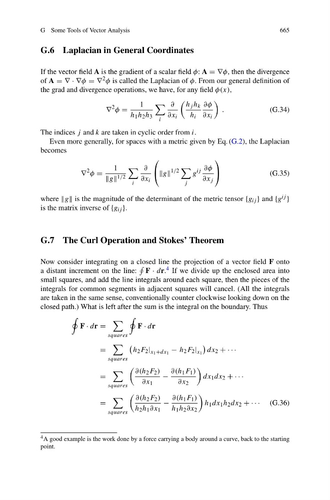
the grad and divergence operations, we have, for any field φ(x),
∇
2 φ =
1
h 1 h 2 h 3
i
∂
∂x i
h j h k
h i
∂φ
∂x i
.
(G.34)
The indices j and k are taken in cyclic order from i.
Even more generally, for spaces with a metric given by Eq. (G.2), the Laplacian
becomes
∇
2 φ =
1
g 1/2
i
∂
∂x i
⎛
⎝ g
1/2
j
g
ij ∂φ
∂x j
⎞
⎠
(G.35)
where g is the magnitude of the determinant of the metric tensor {g ij } and {g ij }
is the matrix inverse of {g ij }.
G.7 The Curl Operation and Stokes’ Theorem
Now consider integrating on a closed line the projection of a vector field F onto
a distant increment on the line:
F · dr. 4 If we divide up the enclosed area into
small squares, and add the line integrals around each square, then the pieces of the
integrals for common segments in adjacent squares will cancel. (All the integrals
are taken in the same sense, conventionally counter clockwise looking down on the
closed path.) What is left after the sum is the integral on the boundary. Thus
F · dr =
squares
F · dr
=
squares
h 2 F 2 | x 1 +dx 1 − h 2 F 2 | x 1
dx 2 + · · ·
=
squares
∂(h 2 F 2 )
∂x 1
−
∂(h 1 F 1 )
∂x 2
dx 1 dx 2 + · · ·
=
squares
∂(h 2 F 2 )
h 2 h 1 ∂x 1
−
∂(h 1 F 1 )
h 1 h 2 ∂x 2
h 1 dx 1 h 2 dx 2 + · · · (G.36)
4 A good example is the work done by a force carrying a body around a curve, back to the starting
point.