

588
14 Neural Networks and Brains
p ∞ =
α
α + β
,
(14.6)
with a time constant of
τ ≡ 1/(α + β) .
(14.7)
The gate-open probability expression Eq. (14.5) applies to all three of the
Hodgkin–Huxley gate probabilities m, h, and n, with different rates for each, except
that for h, which gives the probability of the sodium inactivation gate being open,
the rates α and β reverse roles.
The next task for Hodgkin and Huxley was to find the electric field dependence
of the rates α and β for each of the gates. To do this, they measured the
externally injected current I through the membrane that would hold voltage V
across the membrane fixed at selected values (‘voltage clamped’ measurements).
They could also vary the exterior concentration of potassium and sodium, affecting
the corresponding gated channels. In this way, they could measure the values of m,
n, and h as well as their associated time constants τ , and then solve for the αs and
βs. By plotting these rates as a function of V , they could see that the α and β showed
what appeared to be simple exponential behavior. At the time, they had insufficient
knowledge to support an explanation based on physical principles. To proceed, they
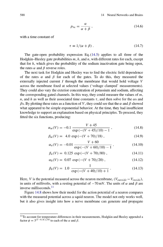
fitted the six functions, producing:
α m (V ) = −0.1
V + 45
exp (−(V + 45)/10) − 1
,
(14.8)
β m (V ) = 4.0 exp (−(V + 70)/18) ,
(14.9)
α n (V ) = −0.01
V + 60
exp (−(V + 60)/10) − 1
,
(14.10)
β n (V ) = 0.125 exp (−(V + 70)/80) ,
(14.11)
α h (V ) = 0.07 exp (−(V + 70)/20) ,
(14.12)
β h (V ) = 1.0
1
exp (−(V + 40)/10) + 1
.
(14.13)
Here, V is the potential measured across the neuron membrane, (V outside − V inside ),
in units of millivolts, with a resting potential of −70 mV. The units of α and β are
inverse milliseconds. 11
Figure 14.8 shows how their model for the action potential of a neuron compares
with the measured potential across a squid neuron. The model not only works well,
but it also gives insight into how a nerve membrane can generate and propagate
11 To account for temperature differences in their measurements, Hodgkin and Huxley appended a
factor φ = 3 (T −6.3C)/10 to each of the α and β.