

580
14 Neural Networks and Brains
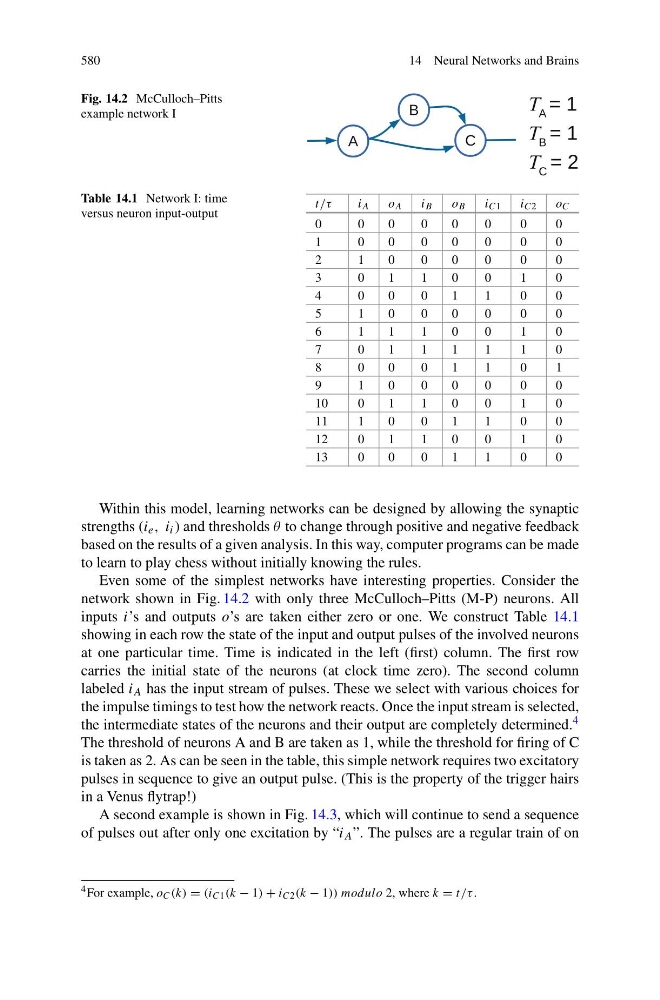
Fig. 14.2 McCulloch–Pitts
example network I
Table 14.1 Network I: time
versus neuron input-output
t/τ
i A
o A
i B
o B
i C1
i C2
o C
0
0
0
0
0
0
0
0
1
0
0
0
0
0
0
0
2
1
0
0
0
0
0
0
3
0
1
1
0
0
1
0
4
0
0
0
1
1
0
0
5
1
0
0
0
0
0
0
6
1
1
1
0
0
1
0
7
0
1
1
1
1
1
0
8
0
0
0
1
1
0
1
9
1
0
0
0
0
0
0
10
0
1
1
0
0
1
0
11
1
0
0
1
1
0
0
12
0
1
1
0
0
1
0
13
0
0
0
1
1
0
0
Within this model, learning networks can be designed by allowing the synaptic
strengths (i e , i i ) and thresholds θ to change through positive and negative feedback
based on the results of a given analysis. In this way, computer programs can be made
to learn to play chess without initially knowing the rules.
Even some of the simplest networks have interesting properties. Consider the
network shown in Fig. 14.2 with only three McCulloch–Pitts (M-P) neurons. All
inputs i’s and outputs o’s are taken either zero or one. We construct Table 14.1
showing in each row the state of the input and output pulses of the involved neurons
at one particular time. Time is indicated in the left (first) column. The first row
carries the initial state of the neurons (at clock time zero). The second column
labeled i A has the input stream of pulses. These we select with various choices for
the impulse timings to test how the network reacts. Once the input stream is selected,
the intermediate states of the neurons and their output are completely determined. 4
The threshold of neurons A and B are taken as 1, while the threshold for firing of C
is taken as 2. As can be seen in the table, this simple network requires two excitatory
pulses in sequence to give an output pulse. (This is the property of the trigger hairs
in a Venus flytrap!)
A second example is shown in Fig. 14.3, which will continue to send a sequence
of pulses out after only one excitation by “i A ”. The pulses are a regular train of on
4 For example, o C (k) = (i C1 (k − 1) + i C2 (k − 1)) modulo 2, where k = t/τ .