

13.3 Optimality Conditions
567
the Fermat point. It turns out that lines from the distal third vertices of the equilateral
triangles to the opposite vertex of the Fermat triangle will also intersect at the
Fermat point. In 1750, Thomas Simpson showed how to generalize this geometric
construction in the case of weighted lengths.
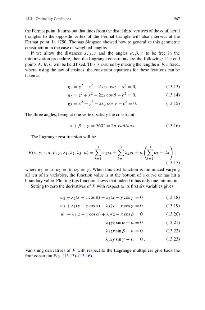
If we allow the distances x, y, z and the angles α, β, γ to be free in the
minimization procedure, then the Lagrange constraints are the following: The end
points A, B, C will be held fixed. This is assured by making the lengths a, b, c fixed,
where, using the law of cosines, the constraint equations for these fixations can be
taken as
g 1 = y
2
+ z
2
− 2yz cos α − a
2
= 0,
(13.13)
g 2 = z
2
+ x
2
− 2zx cos β − b
2
= 0,
(13.14)
g 3 = x
2
+ y
2
− 2xy cos γ − c
2
= 0.
(13.15)
The three angles, being at one vertex, satisfy the constraint
α + β + γ = 360
◦
= 2π radians.
(13.16)
The Lagrange cost function will be
F (x, y, z, α, β, γ, λ 1 , λ 2 , λ 3 , μ) =
3
k=1
w k x k +
3
k=1
λ k g k + μ
3
k=1
α k − 2π
,
(13.17)
where α 1 = α, α 2 = β, α 3 = γ . When this cost function is minimized varying
all ten of its variables, the function value is at the bottom of a curve or has hit a
boundary value. Plotting this function shows that indeed it has only one minimum.
Setting to zero the derivatives of F with respect to its first six variables gives
w 2 + λ 2 (x − z cos β) + λ 3 (x − y cos γ = 0
(13.18)
w 3 + λ 1 (y − z cos α) + λ 3 (y − x cos γ = 0
(13.19)
w 1 + λ 1 (z − y cos α) + λ 2 (z − x cos β = 0
(13.20)
λ 1 yz sin α + μ = 0
(13.21)
λ 2 zx sin β + μ = 0
(13.22)
λ 3 xy sin γ + μ = 0 .
(13.23)
Vanishing derivatives of F with respect to the Lagrange multipliers give back the
four constraint Eqs. (13.13)–(13.16).