

4.3 Fluid Dynamics
107
= −
∇ · (ρv) dV +
∇ · (ρv))dV
= −
∇ · (ρv) dV −
∂ρ
∂t
= −
d
dt
ρρ dV +
ρ
∂∂
∂t
dV .
(4.58)
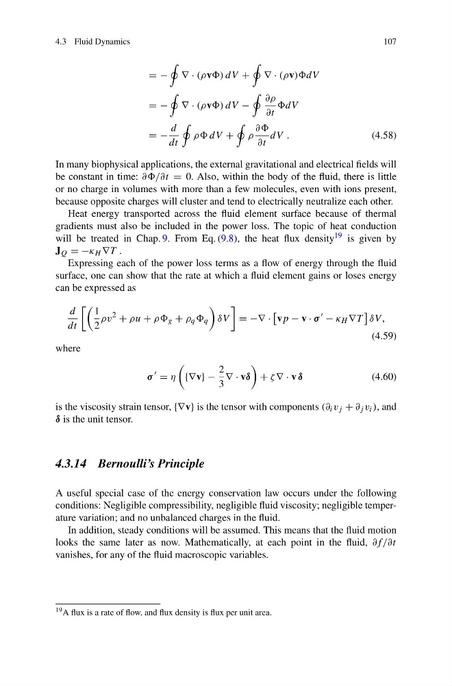
In many biophysical applications, the external gravitational and electrical fields will
be constant in time: ∂∂/∂t = 0. Also, within the body of the fluid, there is little
or no charge in volumes with more than a few molecules, even with ions present,
because opposite charges will cluster and tend to electrically neutralize each other.
Heat energy transported across the fluid element surface because of thermal
gradients must also be included in the power loss. The topic of heat conduction
will be treated in Chap. 9. From Eq. (9.8), the heat flux density 19 is given by
J Q = −κ H ∇T .
Expressing each of the power loss terms as a flow of energy through the fluid
surface, one can show that the rate at which a fluid element gains or loses energy
can be expressed as
d
dt
1
2
ρv
2
+ ρu + ρρ g + ρ q q
δV
= −∇ ·
vp − v · σ
− κ H ∇T
δV ,
(4.59)
where
σ
= η
{∇v} −
2
3
∇ · vδ
+ ζ ∇ · v δ
(4.60)
is the viscosity strain tensor, {∇v} is the tensor with components (∂ i v j + ∂ j v i ), and
δ is the unit tensor.
4.3.14 Bernoulli’s Principle
A useful special case of the energy conservation law occurs under the following
conditions: Negligible compressibility, negligible fluid viscosity; negligible temperature variation; and no unbalanced charges in the fluid.
In addition, steady conditions will be assumed. This means that the fluid motion
looks the same later as now. Mathematically, at each point in the fluid, ∂f/∂t
vanishes, for any of the fluid macroscopic variables.
19 A flux is a rate of flow, and flux density is flux per unit area.
107
= −
∇ · (ρv) dV +
∇ · (ρv))dV
= −
∇ · (ρv) dV −
∂ρ
∂t
= −
d
dt
ρρ dV +
ρ
∂∂
∂t
dV .
(4.58)
In many biophysical applications, the external gravitational and electrical fields will
be constant in time: ∂∂/∂t = 0. Also, within the body of the fluid, there is little
or no charge in volumes with more than a few molecules, even with ions present,
because opposite charges will cluster and tend to electrically neutralize each other.
Heat energy transported across the fluid element surface because of thermal
gradients must also be included in the power loss. The topic of heat conduction
will be treated in Chap. 9. From Eq. (9.8), the heat flux density 19 is given by
J Q = −κ H ∇T .
Expressing each of the power loss terms as a flow of energy through the fluid
surface, one can show that the rate at which a fluid element gains or loses energy
can be expressed as
d
dt
1
2
ρv
2
+ ρu + ρρ g + ρ q q
δV
= −∇ ·
vp − v · σ
− κ H ∇T
δV ,
(4.59)
where
σ
= η
{∇v} −
2
3
∇ · vδ
+ ζ ∇ · v δ
(4.60)
is the viscosity strain tensor, {∇v} is the tensor with components (∂ i v j + ∂ j v i ), and
δ is the unit tensor.
4.3.14 Bernoulli’s Principle
A useful special case of the energy conservation law occurs under the following
conditions: Negligible compressibility, negligible fluid viscosity; negligible temperature variation; and no unbalanced charges in the fluid.
In addition, steady conditions will be assumed. This means that the fluid motion
looks the same later as now. Mathematically, at each point in the fluid, ∂f/∂t
vanishes, for any of the fluid macroscopic variables.
19 A flux is a rate of flow, and flux density is flux per unit area.