

44
3 String Theory
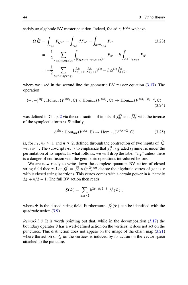
satisfy an algebraic BV master equation. Indeed, for A ∈ V ⊗n we have
Q ˆ
f
g
n =
ν g,n
F QA =
ν g,n
dF A =
∂ geo ν g,n
F A
(3.23)
= −
1
2
n 1 ≤n 2 ;g 1 ≤g 2
{ν g 1 ,n 1 +1 ,ν g 2 ,n 2 +1 } geo
F A − ¯
h
Δ geo ν g,n+2
F A
= −
1
2
n 1 ≤n 2 ;g 1 ≤g 2
{ ˆ
f
g 1
n 1 +1 , ˆ
f
g 2
n 2 +1 }
alg
− ¯
hΔ
alg ˆ
f
g
n+2 ,
where we used in the second line the geometric BV master equation (3.17). The
operation
{−, −}
alg
: Hom inv (V
⊗n 1 , C) × Hom inv (V
⊗n 2 , C) → Hom inv (V
⊗n 1 +n 2 −2 , C)
(3.24)
was defined in Chap. 2 via the contraction of inputs of ˆ
f
g 1
n 1 and ˆ
f
g 2
n 2 with the inverse
of the symplectic form ω. Similarly,
Δ
alg
: Hom inv (V
⊗n , C) → Hom inv (V
⊗n−2 , C)
(3.25)
is, for n 1 , n 2 ≥ 1, and n ≥ 2, defined through the contraction of two inputs of ˆ
f
g
n
with ω −1 . The subscript inv is to emphasize that ˆ
f
g
n is graded symmetric under the
permutation of its inputs. In what follows, we will drop the label “alg” unless there
is a danger of confusion with the geometric operations introduced before.
We are now ready to write down the complete quantum BV action of closed
string field theory. Let f
g
n = ˆ
f
g
n ◦ (↑ 2 ) ⊗n denote the algebraic vertex of genus g
with n closed string insertions. This vertex comes with a certain power in ¯
h, namely
2g + n/2 − 1. The full BV action then reads
S(Ψ ) =
g,n≥2
¯
h
2g+n/2−1 f
g
n (Ψ ) ,
where Ψ is the closed string field. Furthermore, f
0
2 (Ψ ) can be identified with the
quadratic action (3.9).
Remark 3.3 It is worth pointing out that, while in the decomposition (3.17) the
boundary operator ∂ has a well-defined action on the vertices, it does not act on the
punctures. This distinction does not appear on the image of the chain map (3.21)
where the action of Q on the vertices is induced by its action on the vector space
attached to the puncture.
3 String Theory
satisfy an algebraic BV master equation. Indeed, for A ∈ V ⊗n we have
Q ˆ
f
g
n =
ν g,n
F QA =
ν g,n
dF A =
∂ geo ν g,n
F A
(3.23)
= −
1
2
n 1 ≤n 2 ;g 1 ≤g 2
{ν g 1 ,n 1 +1 ,ν g 2 ,n 2 +1 } geo
F A − ¯
h
Δ geo ν g,n+2
F A
= −
1
2
n 1 ≤n 2 ;g 1 ≤g 2
{ ˆ
f
g 1
n 1 +1 , ˆ
f
g 2
n 2 +1 }
alg
− ¯
hΔ
alg ˆ
f
g
n+2 ,
where we used in the second line the geometric BV master equation (3.17). The
operation
{−, −}
alg
: Hom inv (V
⊗n 1 , C) × Hom inv (V
⊗n 2 , C) → Hom inv (V
⊗n 1 +n 2 −2 , C)
(3.24)
was defined in Chap. 2 via the contraction of inputs of ˆ
f
g 1
n 1 and ˆ
f
g 2
n 2 with the inverse
of the symplectic form ω. Similarly,
Δ
alg
: Hom inv (V
⊗n , C) → Hom inv (V
⊗n−2 , C)
(3.25)
is, for n 1 , n 2 ≥ 1, and n ≥ 2, defined through the contraction of two inputs of ˆ
f
g
n
with ω −1 . The subscript inv is to emphasize that ˆ
f
g
n is graded symmetric under the
permutation of its inputs. In what follows, we will drop the label “alg” unless there
is a danger of confusion with the geometric operations introduced before.
We are now ready to write down the complete quantum BV action of closed
string field theory. Let f
g
n = ˆ
f
g
n ◦ (↑ 2 ) ⊗n denote the algebraic vertex of genus g
with n closed string insertions. This vertex comes with a certain power in ¯
h, namely
2g + n/2 − 1. The full BV action then reads
S(Ψ ) =
g,n≥2
¯
h
2g+n/2−1 f
g
n (Ψ ) ,
where Ψ is the closed string field. Furthermore, f
0
2 (Ψ ) can be identified with the
quadratic action (3.9).
Remark 3.3 It is worth pointing out that, while in the decomposition (3.17) the
boundary operator ∂ has a well-defined action on the vertices, it does not act on the
punctures. This distinction does not appear on the image of the chain map (3.21)
where the action of Q on the vertices is induced by its action on the vector space
attached to the puncture.