

426
22 Layered Structures
2600
2620
2640
2660
2680
(cm
-1
)
k' = 0.30; = 1
k' = 0.30; = 0.31
0.0 0.2 0.4 0.6 0.8 1.0 1.2
0.0
0.5
1.0
1.5
2.0
376
378
380
382
384
386
(cm
-1
)
MoS 2
= 0.24, = 0.12
= 0.24, = 1.0
E
+
2g
E
-
2g
(a)
(b)
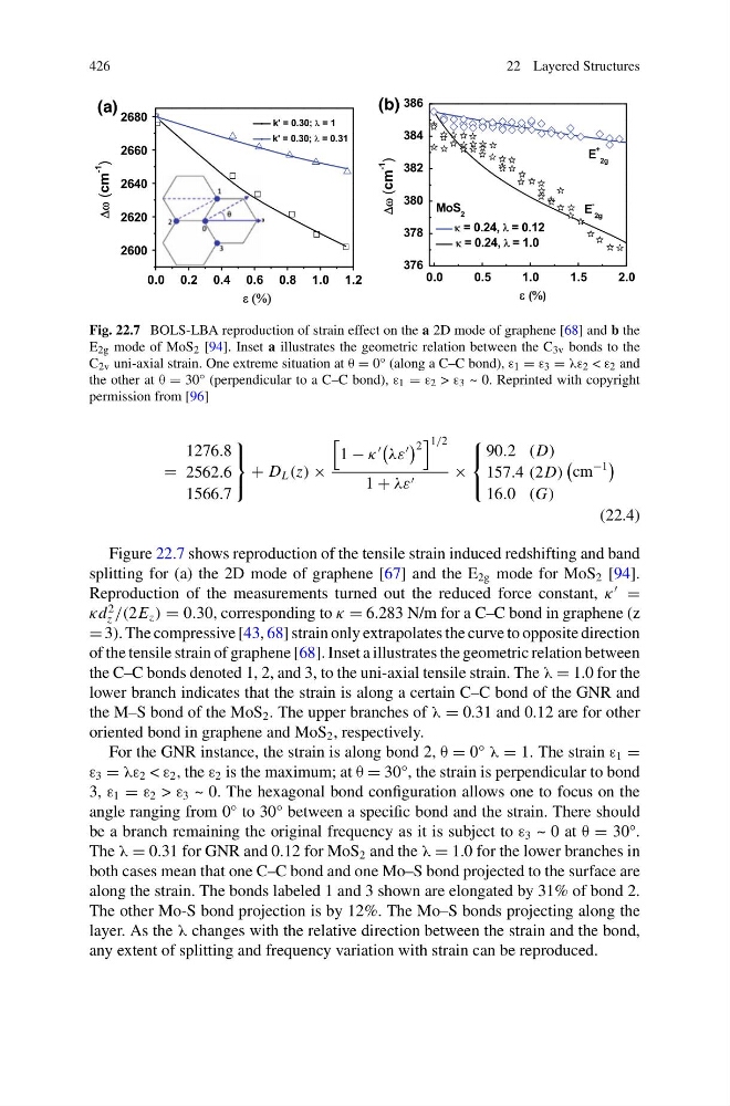
Fig. 22.7 BOLS-LBA reproduction of strain effect on the a 2D mode of graphene [68] and b the
E 2g mode of MoS 2 [94]. Inset a illustrates the geometric relation between the C 3v bonds to the
C 2v uni-axial strain. One extreme situation at θ = 0° (along a C–C bond), ε 1 = ε 3 = λε 2 < ε 2 and
the other at θ = 30° (perpendicular to a C–C bond), ε 1 = ε 2 > ε 3 ~ 0. Reprinted with copyright
permission from [96]
=
1276.8
2562.6
1566.7
⎫
⎬
⎭
+ D L (z) ×
1 − κ
λε
2
1/2
1 + λε
×
⎧
⎨
⎩
90.2 (D)
157.4 (2D)
16.0 (G)
cm
−1
(22.4)
Figure 22.7 shows reproduction of the tensile strain induced redshifting and band
splitting for (a) the 2D mode of graphene [67] and the E 2g mode for MoS 2 [94].
Reproduction of the measurements turned out the reduced force constant, κ
=
κd
2
z /(2E z ) = 0.30, corresponding to κ = 6.283 N/m for a C–C bond in graphene (z
= 3). The compressive [43, 68] strain only extrapolates the curve to opposite direction
of the tensile strain of graphene [68]. Inset a illustrates the geometric relation between
the C–C bonds denoted 1, 2, and 3, to the uni-axial tensile strain. The λ = 1.0 for the
lower branch indicates that the strain is along a certain C–C bond of the GNR and
the M–S bond of the MoS 2 . The upper branches of λ = 0.31 and 0.12 are for other
oriented bond in graphene and MoS 2 , respectively.
For the GNR instance, the strain is along bond 2, θ = 0° λ = 1. The strain ε 1 =
ε 3 = λε 2 < ε 2 , the ε 2 is the maximum; at θ = 30°, the strain is perpendicular to bond
3, ε 1 = ε 2 > ε 3 ~ 0. The hexagonal bond configuration allows one to focus on the
angle ranging from 0° to 30° between a specific bond and the strain. There should
be a branch remaining the original frequency as it is subject to ε 3 ~ 0 at θ = 30°.
The λ = 0.31 for GNR and 0.12 for MoS 2 and the λ = 1.0 for the lower branches in
both cases mean that one C–C bond and one Mo–S bond projected to the surface are
along the strain. The bonds labeled 1 and 3 shown are elongated by 31% of bond 2.
The other Mo-S bond projection is by 12%. The Mo–S bonds projecting along the
layer. As the λ changes with the relative direction between the strain and the bond,
any extent of splitting and frequency variation with strain can be reproduced.
22 Layered Structures
2600
2620
2640
2660
2680
(cm
-1
)
k' = 0.30; = 1
k' = 0.30; = 0.31
0.0 0.2 0.4 0.6 0.8 1.0 1.2
0.0
0.5
1.0
1.5
2.0
376
378
380
382
384
386
(cm
-1
)
MoS 2
= 0.24, = 0.12
= 0.24, = 1.0
E
+
2g
E
-
2g
(a)
(b)
Fig. 22.7 BOLS-LBA reproduction of strain effect on the a 2D mode of graphene [68] and b the
E 2g mode of MoS 2 [94]. Inset a illustrates the geometric relation between the C 3v bonds to the
C 2v uni-axial strain. One extreme situation at θ = 0° (along a C–C bond), ε 1 = ε 3 = λε 2 < ε 2 and
the other at θ = 30° (perpendicular to a C–C bond), ε 1 = ε 2 > ε 3 ~ 0. Reprinted with copyright
permission from [96]
=
1276.8
2562.6
1566.7
⎫
⎬
⎭
+ D L (z) ×
1 − κ
λε
2
1/2
1 + λε
×
⎧
⎨
⎩
90.2 (D)
157.4 (2D)
16.0 (G)
cm
−1
(22.4)
Figure 22.7 shows reproduction of the tensile strain induced redshifting and band
splitting for (a) the 2D mode of graphene [67] and the E 2g mode for MoS 2 [94].
Reproduction of the measurements turned out the reduced force constant, κ
=
κd
2
z /(2E z ) = 0.30, corresponding to κ = 6.283 N/m for a C–C bond in graphene (z
= 3). The compressive [43, 68] strain only extrapolates the curve to opposite direction
of the tensile strain of graphene [68]. Inset a illustrates the geometric relation between
the C–C bonds denoted 1, 2, and 3, to the uni-axial tensile strain. The λ = 1.0 for the
lower branch indicates that the strain is along a certain C–C bond of the GNR and
the M–S bond of the MoS 2 . The upper branches of λ = 0.31 and 0.12 are for other
oriented bond in graphene and MoS 2 , respectively.
For the GNR instance, the strain is along bond 2, θ = 0° λ = 1. The strain ε 1 =
ε 3 = λε 2 < ε 2 , the ε 2 is the maximum; at θ = 30°, the strain is perpendicular to bond
3, ε 1 = ε 2 > ε 3 ~ 0. The hexagonal bond configuration allows one to focus on the
angle ranging from 0° to 30° between a specific bond and the strain. There should
be a branch remaining the original frequency as it is subject to ε 3 ~ 0 at θ = 30°.
The λ = 0.31 for GNR and 0.12 for MoS 2 and the λ = 1.0 for the lower branches in
both cases mean that one C–C bond and one Mo–S bond projected to the surface are
along the strain. The bonds labeled 1 and 3 shown are elongated by 31% of bond 2.
The other Mo-S bond projection is by 12%. The Mo–S bonds projecting along the
layer. As the λ changes with the relative direction between the strain and the bond,
any extent of splitting and frequency variation with strain can be reproduced.