

and a current metastable-state population α(t), Eqs. (1 and 4) can be rearranged to
obtain the effective time t
0 capturing the progress of the two processes:
α t
ð Þ ¼ 1 À exp Àk exc t
0
exc
À
Á ⟹t
0
exc ¼ À
1
k exc
ln 1 À α t
ð Þ
½
ð 10Þ
α t
ð Þ ¼ exp Àk dec t
0
dec
À
Á
⟹t
0
dec ¼ À
1
k dec
ln α t
ð Þ
ð11Þ
Here, we have distinguished the k and t
0 for the two processes with subscript dec
and exc and assumed n ¼ 1 for simplicity.
Having obtained t
0
exc and t
0
dec , we can then predict the change in excited-state
population Δα over the time interval t ! t + Δt as follows:
Δα t ! t þ Δt
ð
Þ¼ 1 À exp Àk exc t
0
exc þ Δt
À
Á
Â
à À α t
ð Þ
È
É
À α t
ð Þ À exp Àk dec t
0
dec þ Δt
À
Á
Â
Ã
È
É
ð12Þ
The first term in braces calculates the growth in excited-state population over the
interval due to excitation, while the second term calculates the reduction in population due to decay. An adjustment is then applied to clamp α(t) to the range [0, 1].
Provided a sufficiently small Δt is chosen, these simulations provide a good description of the time evolution of the excited-state population for a given set of conditions.
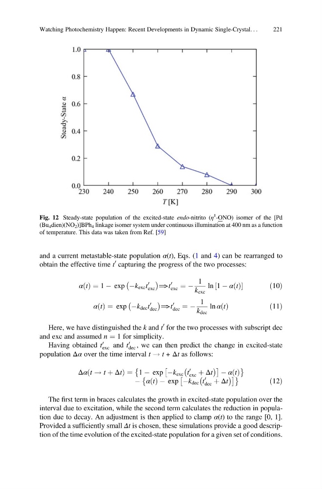
Fig. 12 Steady-state population of the excited-state endo-nitrito (η
1
-ONO) isomer of the [Pd
(Bu 4 dien)(NO 2 )]BPh 4 linkage isomer system under continuous illumination at 400 nm as a function
of temperature. This data was taken from Ref. [59]
Watching Photochemistry Happen: Recent Developments in Dynamic Single-Crystal. . .
221
obtain the effective time t
0 capturing the progress of the two processes:
α t
ð Þ ¼ 1 À exp Àk exc t
0
exc
À
Á ⟹t
0
exc ¼ À
1
k exc
ln 1 À α t
ð Þ
½
ð 10Þ
α t
ð Þ ¼ exp Àk dec t
0
dec
À
Á
⟹t
0
dec ¼ À
1
k dec
ln α t
ð Þ
ð11Þ
Here, we have distinguished the k and t
0 for the two processes with subscript dec
and exc and assumed n ¼ 1 for simplicity.
Having obtained t
0
exc and t
0
dec , we can then predict the change in excited-state
population Δα over the time interval t ! t + Δt as follows:
Δα t ! t þ Δt
ð
Þ¼ 1 À exp Àk exc t
0
exc þ Δt
À
Á
Â
à À α t
ð Þ
È
É
À α t
ð Þ À exp Àk dec t
0
dec þ Δt
À
Á
Â
Ã
È
É
ð12Þ
The first term in braces calculates the growth in excited-state population over the
interval due to excitation, while the second term calculates the reduction in population due to decay. An adjustment is then applied to clamp α(t) to the range [0, 1].
Provided a sufficiently small Δt is chosen, these simulations provide a good description of the time evolution of the excited-state population for a given set of conditions.
Fig. 12 Steady-state population of the excited-state endo-nitrito (η
1
-ONO) isomer of the [Pd
(Bu 4 dien)(NO 2 )]BPh 4 linkage isomer system under continuous illumination at 400 nm as a function
of temperature. This data was taken from Ref. [59]
Watching Photochemistry Happen: Recent Developments in Dynamic Single-Crystal. . .
221