

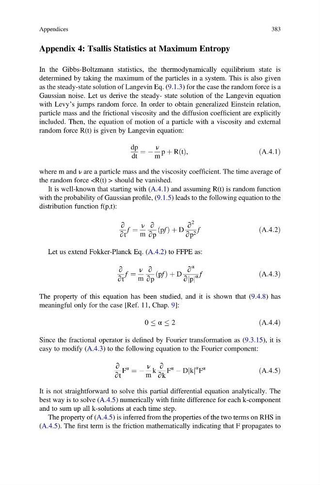
Appendix 4: Tsallis Statistics at Maximum Entropy
In the Gibbs-Boltzmann statistics, the thermodynamically equilibrium state is
determined by taking the maximum of the particles in a system. This is also given
as the steady-state solution of Langevin Eq. (9.1.3) for the case the random force is a
Gaussian noise. Let us derive the steady- state solution of the Langevin equation
with Levy’s jumps random force. In order to obtain generalized Einstein relation,
particle mass and the frictional viscosity and the diffusion coefficient are explicitly
included. Then, the equation of motion of a particle with a viscosity and external
random force R(t) is given by Langevin equation:
dp
dt
¼ À
ν
m
p þ R t
ð Þ,
ðA:4:1Þ
where m and ν are a particle mass and the viscosity coefficient. The time average of
the random force should be vanished.
It is well-known that starting with (A.4.1) and assuming R(t) is random function
with the probability of Gaussian profile, (9.1.5) leads to the following equation to the
distribution function f(p,t):
∂
∂t
f ¼
ν
m
∂
∂p
pf
ð Þ þ D
∂
2
∂p 2 f
ðA:4:2Þ
Let us extend Fokker-Planck Eq. (A.4.2) to FFPE as:
∂
∂t
f ¼
ν
m
∂
∂p
pf
ð Þ þ D
∂
α
∂ p
j j
α f
ðA:4:3Þ
The property of this equation has been studied, and it is shown that (9.4.8) has
meaningful only for the case [Ref. 11, Chap. 9]:
0 α 2
ðA:4:4Þ
Since the fractional operator is defined by Fourier transformation as (9.3.15), it is
easy to modify (A.4.3) to the following equation to the Fourier component:
∂
∂t
F
α
¼ À
ν
m
k
∂
∂k
F
α
À D k
j j
α F
α
ðA:4:5Þ
It is not straightforward to solve this partial differential equation analytically. The
best way is to solve (A.4.5) numerically with finite difference for each k-component
and to sum up all k-solutions at each time step.
The property of (A.4.5) is inferred from the properties of the two terms on RHS in
(A.4.5). The first term is the friction mathematically indicating that F propagates to
Appendices
383
In the Gibbs-Boltzmann statistics, the thermodynamically equilibrium state is
determined by taking the maximum of the particles in a system. This is also given
as the steady-state solution of Langevin Eq. (9.1.3) for the case the random force is a
Gaussian noise. Let us derive the steady- state solution of the Langevin equation
with Levy’s jumps random force. In order to obtain generalized Einstein relation,
particle mass and the frictional viscosity and the diffusion coefficient are explicitly
included. Then, the equation of motion of a particle with a viscosity and external
random force R(t) is given by Langevin equation:
dp
dt
¼ À
ν
m
p þ R t
ð Þ,
ðA:4:1Þ
where m and ν are a particle mass and the viscosity coefficient. The time average of
the random force
It is well-known that starting with (A.4.1) and assuming R(t) is random function
with the probability of Gaussian profile, (9.1.5) leads to the following equation to the
distribution function f(p,t):
∂
∂t
f ¼
ν
m
∂
∂p
pf
ð Þ þ D
∂
2
∂p 2 f
ðA:4:2Þ
Let us extend Fokker-Planck Eq. (A.4.2) to FFPE as:
∂
∂t
f ¼
ν
m
∂
∂p
pf
ð Þ þ D
∂
α
∂ p
j j
α f
ðA:4:3Þ
The property of this equation has been studied, and it is shown that (9.4.8) has
meaningful only for the case [Ref. 11, Chap. 9]:
0 α 2
ðA:4:4Þ
Since the fractional operator is defined by Fourier transformation as (9.3.15), it is
easy to modify (A.4.3) to the following equation to the Fourier component:
∂
∂t
F
α
¼ À
ν
m
k
∂
∂k
F
α
À D k
j j
α F
α
ðA:4:5Þ
It is not straightforward to solve this partial differential equation analytically. The
best way is to solve (A.4.5) numerically with finite difference for each k-component
and to sum up all k-solutions at each time step.
The property of (A.4.5) is inferred from the properties of the two terms on RHS in
(A.4.5). The first term is the friction mathematically indicating that F propagates to
Appendices
383