

Appendix-3: PIC Simulation
It is well-known that from the begging of the invention of computers in the 1950s,
plasma physics has been a pioneering field to advance the computation for studying
complex phenomena in science. Plasma physics is many body interaction systems
requiring high-speed computer for a variety of problems to check theory and to
analyze and design experiments. Particle-in-cell (PIC) simulation is a direct
modeling to solve charged particle motions in electric and magnetic fields. The
early works before the 1980s are reviewed by a pioneer of PIC simulation method,
John Dawson, in Ref. [1], where the numerical algorism is also well described.
Particles in Computer
The PIC, a computer simulation for the first principle, is to solve Maxwell Eqs. (1.
3.1), (1.3.2), (1.3.3) and (1.3.4) by coupling with many of particle motions for
electrons and ions governed by (1.3.8) and time integration of velocity to obtain
particle positions:
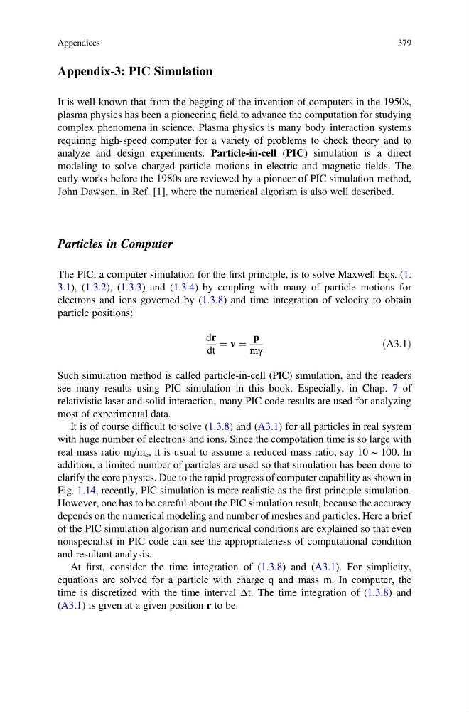
dr
dt
¼ v ¼
p
mγ
ðA3:1Þ
Such simulation method is called particle-in-cell (PIC) simulation, and the readers
see many results using PIC simulation in this book. Especially, in Chap. 7 of
relativistic laser and solid interaction, many PIC code results are used for analyzing
most of experimental data.
It is of course difficult to solve (1.3.8) and (A3.1) for all particles in real system
with huge number of electrons and ions. Since the compotation time is so large with
real mass ratio m i /m e , it is usual to assume a reduced mass ratio, say 10 ~ 100. In
addition, a limited number of particles are used so that simulation has been done to
clarify the core physics. Due to the rapid progress of computer capability as shown in
Fig. 1.14, recently, PIC simulation is more realistic as the first principle simulation.
However, one has to be careful about the PIC simulation result, because the accuracy
depends on the numerical modeling and number of meshes and particles. Here a brief
of the PIC simulation algorism and numerical conditions are explained so that even
nonspecialist in PIC code can see the appropriateness of computational condition
and resultant analysis.
At first, consider the time integration of (1.3.8) and (A3.1). For simplicity,
equations are solved for a particle with charge q and mass m. In computer, the
time is discretized with the time interval Δt. The time integration of (1.3.8) and
(A3.1) is given at a given position r to be:
Appendices
379
It is well-known that from the begging of the invention of computers in the 1950s,
plasma physics has been a pioneering field to advance the computation for studying
complex phenomena in science. Plasma physics is many body interaction systems
requiring high-speed computer for a variety of problems to check theory and to
analyze and design experiments. Particle-in-cell (PIC) simulation is a direct
modeling to solve charged particle motions in electric and magnetic fields. The
early works before the 1980s are reviewed by a pioneer of PIC simulation method,
John Dawson, in Ref. [1], where the numerical algorism is also well described.
Particles in Computer
The PIC, a computer simulation for the first principle, is to solve Maxwell Eqs. (1.
3.1), (1.3.2), (1.3.3) and (1.3.4) by coupling with many of particle motions for
electrons and ions governed by (1.3.8) and time integration of velocity to obtain
particle positions:
dr
dt
¼ v ¼
p
mγ
ðA3:1Þ
Such simulation method is called particle-in-cell (PIC) simulation, and the readers
see many results using PIC simulation in this book. Especially, in Chap. 7 of
relativistic laser and solid interaction, many PIC code results are used for analyzing
most of experimental data.
It is of course difficult to solve (1.3.8) and (A3.1) for all particles in real system
with huge number of electrons and ions. Since the compotation time is so large with
real mass ratio m i /m e , it is usual to assume a reduced mass ratio, say 10 ~ 100. In
addition, a limited number of particles are used so that simulation has been done to
clarify the core physics. Due to the rapid progress of computer capability as shown in
Fig. 1.14, recently, PIC simulation is more realistic as the first principle simulation.
However, one has to be careful about the PIC simulation result, because the accuracy
depends on the numerical modeling and number of meshes and particles. Here a brief
of the PIC simulation algorism and numerical conditions are explained so that even
nonspecialist in PIC code can see the appropriateness of computational condition
and resultant analysis.
At first, consider the time integration of (1.3.8) and (A3.1). For simplicity,
equations are solved for a particle with charge q and mass m. In computer, the
time is discretized with the time interval Δt. The time integration of (1.3.8) and
(A3.1) is given at a given position r to be:
Appendices
379