

p
tþΔt=2
À p
tÀΔt=2
Δt
¼ q E
t
þ
p
mγ
t
 B
t
!
ðA3:2Þ
r
tþΔt
À r
t
Δt
¼
p
mγ
tþΔt=2
ðA3:3Þ
Note that the physical quantities on RHSs in (A3.2) and (A3.3) are located at the
center of time integration in order to keep higher accuracy.
Maxwell Equations in Computer
Calculating the electric current density j as the sum of all particle currents as a
function of space at time t + Δt by the use of (A3.2) and (A3.1), Maxwell Eqs. (1.3.1)
and (1.3.2) have to be also time integrated as:
B
tþΔt
À B
t
Δt
¼ À∇ Â E
tþΔt=2
ðA3:4Þ
ε 0
E
tþΔt
À E
t
Δt
¼
1
μ 0
∇ Â B
tþΔt=2
À j
tþΔt=2
ðA3:5Þ
Inserting given E and B at time t in (A3.2), it is well-known that with this simple
numerical method, the particle energy cannot conserve even without E field, because
of the numerical error. Numerical algorithm called Buneman-Boris method [2] is
widely used to avoid this numerical difficulty and keep the magnetic field gives only
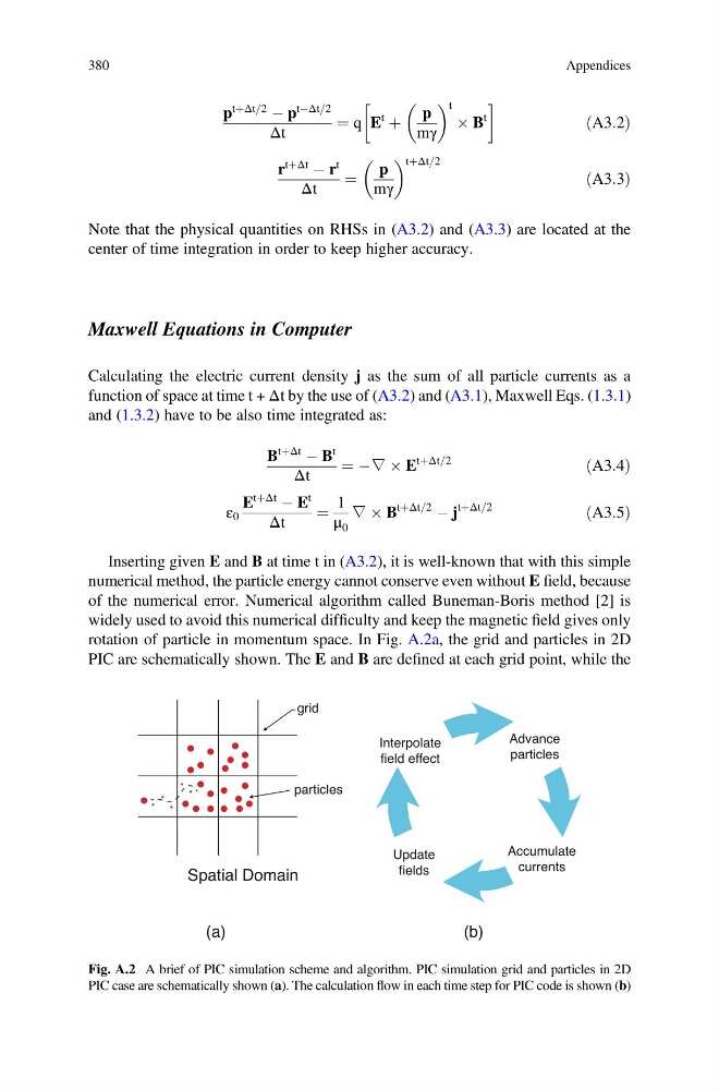
rotation of particle in momentum space. In Fig. A.2a, the grid and particles in 2D
PIC are schematically shown. The E and B are defined at each grid point, while the
grid
particles
Spatial Domain
(a)
(b)
Update
fields
Interpolate
field effect
Advance
particles
Accumulate
currents
Fig. A.2 A brief of PIC simulation scheme and algorithm. PIC simulation grid and particles in 2D
PIC case are schematically shown (a). The calculation flow in each time step for PIC code is shown (b)
380
Appendices
tþΔt=2
À p
tÀΔt=2
Δt
¼ q E
t
þ
p
mγ
t
 B
t
!
ðA3:2Þ
r
tþΔt
À r
t
Δt
¼
p
mγ
tþΔt=2
ðA3:3Þ
Note that the physical quantities on RHSs in (A3.2) and (A3.3) are located at the
center of time integration in order to keep higher accuracy.
Maxwell Equations in Computer
Calculating the electric current density j as the sum of all particle currents as a
function of space at time t + Δt by the use of (A3.2) and (A3.1), Maxwell Eqs. (1.3.1)
and (1.3.2) have to be also time integrated as:
B
tþΔt
À B
t
Δt
¼ À∇ Â E
tþΔt=2
ðA3:4Þ
ε 0
E
tþΔt
À E
t
Δt
¼
1
μ 0
∇ Â B
tþΔt=2
À j
tþΔt=2
ðA3:5Þ
Inserting given E and B at time t in (A3.2), it is well-known that with this simple
numerical method, the particle energy cannot conserve even without E field, because
of the numerical error. Numerical algorithm called Buneman-Boris method [2] is
widely used to avoid this numerical difficulty and keep the magnetic field gives only
rotation of particle in momentum space. In Fig. A.2a, the grid and particles in 2D
PIC are schematically shown. The E and B are defined at each grid point, while the
grid
particles
Spatial Domain
(a)
(b)
Update
fields
Interpolate
field effect
Advance
particles
Accumulate
currents
Fig. A.2 A brief of PIC simulation scheme and algorithm. PIC simulation grid and particles in 2D
PIC case are schematically shown (a). The calculation flow in each time step for PIC code is shown (b)
380
Appendices