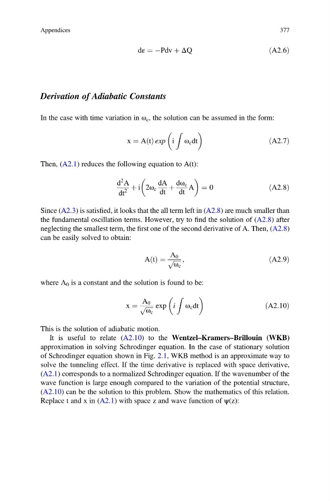
dε ¼ ÀPdv þ ΔQ
ðA2:6Þ
Derivation of Adiabatic Constants
In the case with time variation in ω c , the solution can be assumed in the form:
x ¼ A t
ð Þ exp i
Z
ω c dt
ðA2:7Þ
Then, (A2.1) reduces the following equation to A(t):
d
2 A
dt
2
þ i 2ω c
dA
dt
þ
dω c
dt
A
¼ 0
ðA2:8Þ
Since (A2.3) is satisfied, it looks that the all term left in (A2.8) are much smaller than
the fundamental oscillation terms. However, try to find the solution of (A2.8) after
neglecting the smallest term, the first one of the second derivative of A. Then, (A2.8)
can be easily solved to obtain:
A t
ð Þ ¼
A 0
ffiffiffiffiffi
ω c
p ,
ðA2:9Þ
where A 0 is a constant and the solution is found to be:
x ¼
A 0
ffiffiffiffiffi
ω c
p exp i
Z
ω c dt
ðA2:10Þ
This is the solution of adiabatic motion.
It is useful to relate (A2.10) to the Wentzel–Kramers–Brillouin (WKB)
approximation in solving Schrodinger equation. In the case of stationary solution
of Schrodinger equation shown in Fig. 2.1, WKB method is an approximate way to
solve the tunneling effect. If the time derivative is replaced with space derivative,
(A2.1) corresponds to a normalized Schrodinger equation. If the wavenumber of the
wave function is large enough compared to the variation of the potential structure,
(A2.10) can be the solution to this problem. Show the mathematics of this relation.
Replace t and x in (A2.1) with space z and wave function of ψ(z):
Appendices
377