

8.7.2 One-Electron Orbit
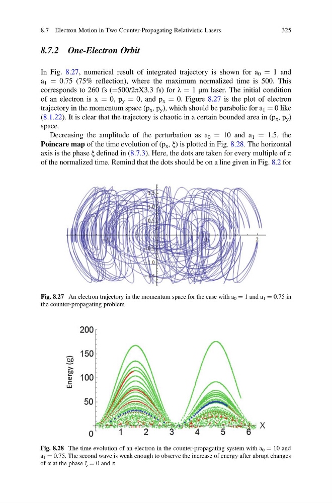
In Fig. 8.27, numerical result of integrated trajectory is shown for a 0 ¼ 1 and
a 1 ¼ 0.75 (75% reflection), where the maximum normalized time is 500. This
corresponds to 260 fs (¼500/2πX3.3 fs) for λ ¼ 1 μm laser. The initial condition
of an electron is x ¼ 0, p y ¼ 0, and p x ¼ 0. Figure 8.27 is the plot of electron
trajectory in the momentum space (p x , p y ), which should be parabolic for a 1 ¼ 0 like
(8.1.22). It is clear that the trajectory is chaotic in a certain bounded area in (p x , p y )
space.
Decreasing the amplitude of the perturbation as a 0 ¼ 10 and a 1 ¼ 1.5, the
Poincare map of the time evolution of (p x , ξ) is plotted in Fig. 8.28. The horizontal
axis is the phase ξ defined in (8.7.3). Here, the dots are taken for every multiple of π
of the normalized time. Remind that the dots should be on a line given in Fig. 8.2 for
Fig. 8.27 An electron trajectory in the momentum space for the case with a 0 ¼ 1 and a 1 ¼ 0.75 in
the counter-propagating problem
Fig. 8.28 The time evolution of an electron in the counter-propagating system with a 0 ¼ 10 and
a 1 ¼ 0.75. The second wave is weak enough to observe the increase of energy after abrupt changes
of α at the phase ξ ¼ 0 and π
8.7 Electron Motion in Two Counter-Propagating Relativistic Lasers
325
In Fig. 8.27, numerical result of integrated trajectory is shown for a 0 ¼ 1 and
a 1 ¼ 0.75 (75% reflection), where the maximum normalized time is 500. This
corresponds to 260 fs (¼500/2πX3.3 fs) for λ ¼ 1 μm laser. The initial condition
of an electron is x ¼ 0, p y ¼ 0, and p x ¼ 0. Figure 8.27 is the plot of electron
trajectory in the momentum space (p x , p y ), which should be parabolic for a 1 ¼ 0 like
(8.1.22). It is clear that the trajectory is chaotic in a certain bounded area in (p x , p y )
space.
Decreasing the amplitude of the perturbation as a 0 ¼ 10 and a 1 ¼ 1.5, the
Poincare map of the time evolution of (p x , ξ) is plotted in Fig. 8.28. The horizontal
axis is the phase ξ defined in (8.7.3). Here, the dots are taken for every multiple of π
of the normalized time. Remind that the dots should be on a line given in Fig. 8.2 for
Fig. 8.27 An electron trajectory in the momentum space for the case with a 0 ¼ 1 and a 1 ¼ 0.75 in
the counter-propagating problem
Fig. 8.28 The time evolution of an electron in the counter-propagating system with a 0 ¼ 10 and
a 1 ¼ 0.75. The second wave is weak enough to observe the increase of energy after abrupt changes
of α at the phase ξ ¼ 0 and π
8.7 Electron Motion in Two Counter-Propagating Relativistic Lasers
325