

j db ¼ À
e
2
mγ 0
δn 2ϕ
ð ÞA ϕ
ð Þ
ð6:2:9Þ
Regarding the third harmonics, the nonlinear current (6.2.9) is almost the same value
as j
R in (6.2.7) [1]. This is shown soon later by calculating both currents explicitly.
In Ref. [1], one-dimensional PIC simulation has also been done to observe the
emission of HHG in under-dense uniform plasmas, where n 0 /n cr ¼ 1/25 is set for
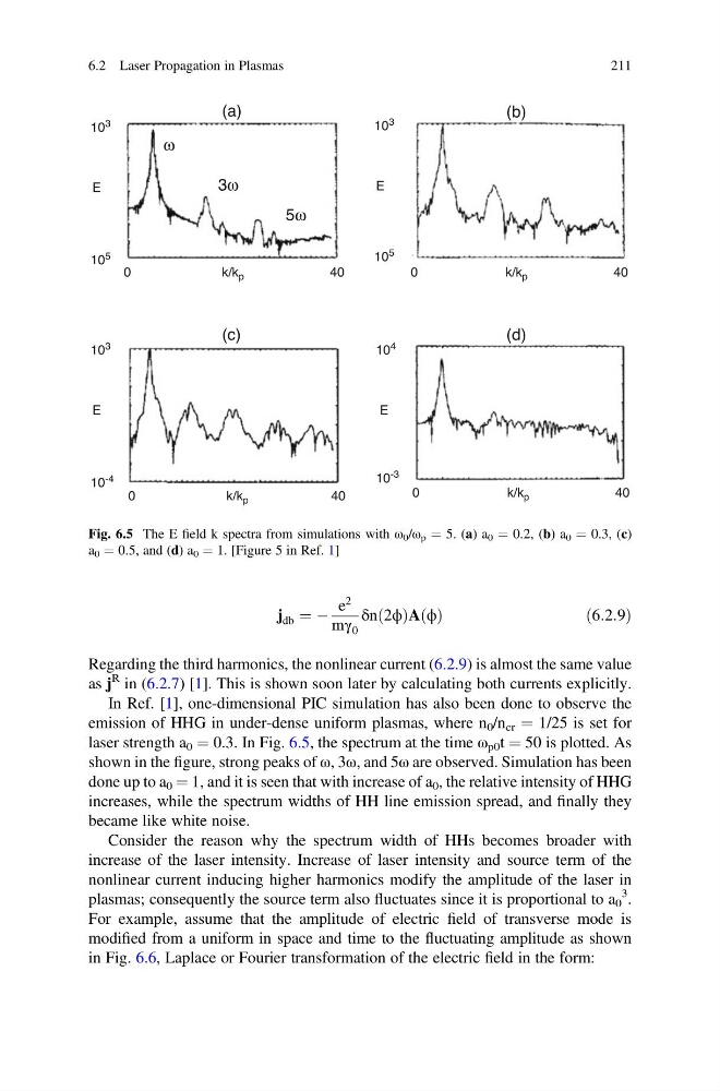
laser strength a 0 ¼ 0.3. In Fig. 6.5, the spectrum at the time ω p0 t ¼ 50 is plotted. As
shown in the figure, strong peaks of ω, 3ω, and 5ω are observed. Simulation has been
done up to a 0 ¼ 1, and it is seen that with increase of a 0 , the relative intensity of HHG
increases, while the spectrum widths of HH line emission spread, and finally they
became like white noise.
Consider the reason why the spectrum width of HHs becomes broader with
increase of the laser intensity. Increase of laser intensity and source term of the
nonlinear current inducing higher harmonics modify the amplitude of the laser in
plasmas; consequently the source term also fluctuates since it is proportional to a 0
3 .
For example, assume that the amplitude of electric field of transverse mode is
modified from a uniform in space and time to the fluctuating amplitude as shown
in Fig. 6.6, Laplace or Fourier transformation of the electric field in the form:
10
3
(a)
(c)
ω
3ω
5ω
(d)
(b)
10
5
0
4 0
k/k p
0
4 0
k/k p
E
10
3
10
4
10 -3
10
-4
E
E
10 3
10
5
0
4 0
k/k p
0
4 0
k/k p
E
Fig. 6.5 The E field k spectra from simulations with ω 0 /ω p ¼ 5. (a) a 0 ¼ 0.2, (b) a 0 ¼ 0.3, (c)
a 0 ¼ 0.5, and (d) a 0 ¼ 1. [Figure 5 in Ref. 1]
6.2 Laser Propagation in Plasmas
211
e
2
mγ 0
δn 2ϕ
ð ÞA ϕ
ð Þ
ð6:2:9Þ
Regarding the third harmonics, the nonlinear current (6.2.9) is almost the same value
as j
R in (6.2.7) [1]. This is shown soon later by calculating both currents explicitly.
In Ref. [1], one-dimensional PIC simulation has also been done to observe the
emission of HHG in under-dense uniform plasmas, where n 0 /n cr ¼ 1/25 is set for
laser strength a 0 ¼ 0.3. In Fig. 6.5, the spectrum at the time ω p0 t ¼ 50 is plotted. As
shown in the figure, strong peaks of ω, 3ω, and 5ω are observed. Simulation has been
done up to a 0 ¼ 1, and it is seen that with increase of a 0 , the relative intensity of HHG
increases, while the spectrum widths of HH line emission spread, and finally they
became like white noise.
Consider the reason why the spectrum width of HHs becomes broader with
increase of the laser intensity. Increase of laser intensity and source term of the
nonlinear current inducing higher harmonics modify the amplitude of the laser in
plasmas; consequently the source term also fluctuates since it is proportional to a 0
3 .
For example, assume that the amplitude of electric field of transverse mode is
modified from a uniform in space and time to the fluctuating amplitude as shown
in Fig. 6.6, Laplace or Fourier transformation of the electric field in the form:
10
3
(a)
(c)
ω
3ω
5ω
(d)
(b)
10
5
0
4 0
k/k p
0
4 0
k/k p
E
10
3
10
4
10 -3
10
-4
E
E
10 3
10
5
0
4 0
k/k p
0
4 0
k/k p
E
Fig. 6.5 The E field k spectra from simulations with ω 0 /ω p ¼ 5. (a) a 0 ¼ 0.2, (b) a 0 ¼ 0.3, (c)
a 0 ¼ 0.5, and (d) a 0 ¼ 1. [Figure 5 in Ref. 1]
6.2 Laser Propagation in Plasmas
211