

and Kruer showed how to obtain approximately the functional dependence of the
driver filed in his textbook (Chap. 2, Ref. [2]).
Kruer assumed the magnitude at the turning point of (3.1.2) can be approximated
with the solution of RHS ¼ 0 in (3.1.2), and in addition, he assumed k 0 L >> 1. Then,
with use of the airy function in Fig. 3.6, the following relation is obtained:
cB z ε ¼ sin
2
θ
À
Á ¼ 0:9E 0 k 0 L
ð
Þ
1=6
ð3:6:6Þ
Then, this value at the turning point is extending by taking account of the attenuation
to the critical point by the tunneling effect. The following attenuation rate e
-β is
obtained by integrating k of (3.1.2):
e
Àβ
: β ¼
2
3
k 0 Lsin
3
θ
ð3:6:7Þ
By the use of (3.6.6) and (3.6.7), we obtain the following function:
E d ¼
E 0
ffiffiffiffiffiffiffiffiffiffiffiffi ffi
2πk 0 L
p
Φ τ
ð Þ
Φ τ
ð Þ ¼ 2:3τ exp À2=3τ
3
À
Á
τ k 0 L
ð
Þ
1=3 sinθ
ð3:6:8Þ
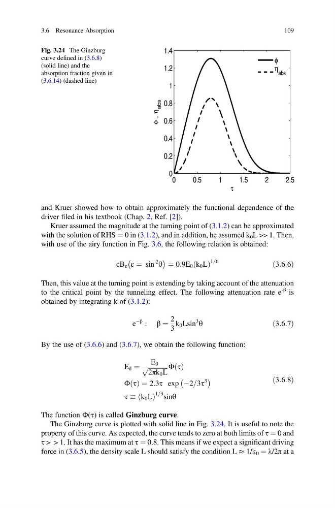
The function Φ(τ) is called Ginzburg curve.
The Ginzburg curve is plotted with solid line in Fig. 3.24. It is useful to note the
property of this curve. As expected, the curve tends to zero at both limits of τ ¼ 0 and
τ > > 1. It has the maximum at τ ¼ 0.8. This means if we expect a significant driving
force in (3.6.5), the density scale L should satisfy the condition L % 1/k 0 ¼ λ/2π at a
Fig. 3.24 The Ginzburg
curve defined in (3.6.8)
(solid line) and the
absorption fraction given in
(3.6.14) (dashed line)
3.6 Resonance Absorption
109
driver filed in his textbook (Chap. 2, Ref. [2]).
Kruer assumed the magnitude at the turning point of (3.1.2) can be approximated
with the solution of RHS ¼ 0 in (3.1.2), and in addition, he assumed k 0 L >> 1. Then,
with use of the airy function in Fig. 3.6, the following relation is obtained:
cB z ε ¼ sin
2
θ
À
Á ¼ 0:9E 0 k 0 L
ð
Þ
1=6
ð3:6:6Þ
Then, this value at the turning point is extending by taking account of the attenuation
to the critical point by the tunneling effect. The following attenuation rate e
-β is
obtained by integrating k of (3.1.2):
e
Àβ
: β ¼
2
3
k 0 Lsin
3
θ
ð3:6:7Þ
By the use of (3.6.6) and (3.6.7), we obtain the following function:
E d ¼
E 0
ffiffiffiffiffiffiffiffiffiffiffiffi ffi
2πk 0 L
p
Φ τ
ð Þ
Φ τ
ð Þ ¼ 2:3τ exp À2=3τ
3
À
Á
τ k 0 L
ð
Þ
1=3 sinθ
ð3:6:8Þ
The function Φ(τ) is called Ginzburg curve.
The Ginzburg curve is plotted with solid line in Fig. 3.24. It is useful to note the
property of this curve. As expected, the curve tends to zero at both limits of τ ¼ 0 and
τ > > 1. It has the maximum at τ ¼ 0.8. This means if we expect a significant driving
force in (3.6.5), the density scale L should satisfy the condition L % 1/k 0 ¼ λ/2π at a
Fig. 3.24 The Ginzburg
curve defined in (3.6.8)
(solid line) and the
absorption fraction given in
(3.6.14) (dashed line)
3.6 Resonance Absorption
109