

where the single particle angular scattering function is computed from the Hapke
parameters from Fornasier et al. (2016).
So that the reflectance from a column density of particles, N d , in units of [# m
À2 ],
under the assumption of negligible optical depth and a single size, is given by
ρ F ¼ ρ sÀd α
ð Þσ x a
ð ÞN d
ð4:110Þ
where ρ s-d is the reflectance of a single particle at a phase angle, α, for which we can
use Fig. 4.16. Combining this equation with Eqs. (4.60) and (4.2) and substituting
for the geometric cross-section with πa
2 we can arrive at
Q d ¼
2
3
Af ρ
v d
ρ sÀd α
ð Þ
a ρ d
ð4:111Þ
If we use 67P as an example again and assume Afρ is 2 m at maximum
(Fig. 4.18), ρ s-d (90
) % 1.5 10
À3 (Fig. 4.16), a ¼ 1 mm, ρ d ¼ 1000 kg m
À3 , and
v d ¼ 2 m/s, then we get Q d ~ 2 10
3 kg s
À1 . This would be at least 2–3 times higher
than the gas production rate (Fig. 3.7) and possibly more given the rather low
estimate for the outflow velocity, v d and therefore giving a dust/gas mass loss rate
ratio much higher than can be tolerated by the measurements of Pätzold et al. (2019).
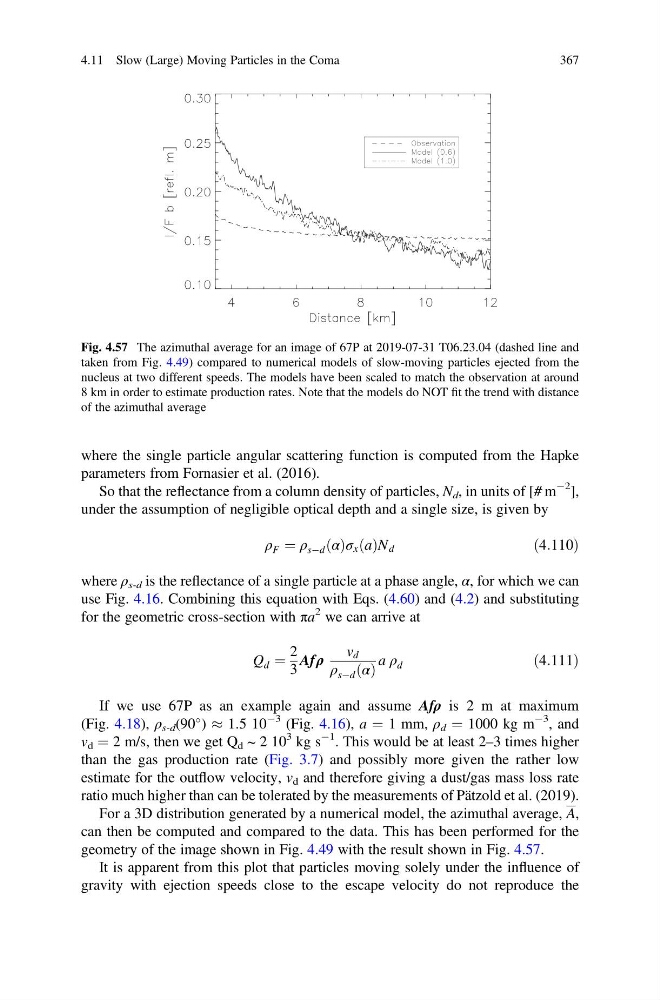
For a 3D distribution generated by a numerical model, the azimuthal average, A,
can then be computed and compared to the data. This has been performed for the
geometry of the image shown in Fig. 4.49 with the result shown in Fig. 4.57.
It is apparent from this plot that particles moving solely under the influence of
gravity with ejection speeds close to the escape velocity do not reproduce the
Fig. 4.57 The azimuthal average for an image of 67P at 2019-07-31 T06.23.04 (dashed line and
taken from Fig. 4.49) compared to numerical models of slow-moving particles ejected from the
nucleus at two different speeds. The models have been scaled to match the observation at around
8 km in order to estimate production rates. Note that the models do NOT fit the trend with distance
of the azimuthal average
4.11 Slow (Large) Moving Particles in the Coma
367
parameters from Fornasier et al. (2016).
So that the reflectance from a column density of particles, N d , in units of [# m
À2 ],
under the assumption of negligible optical depth and a single size, is given by
ρ F ¼ ρ sÀd α
ð Þσ x a
ð ÞN d
ð4:110Þ
where ρ s-d is the reflectance of a single particle at a phase angle, α, for which we can
use Fig. 4.16. Combining this equation with Eqs. (4.60) and (4.2) and substituting
for the geometric cross-section with πa
2 we can arrive at
Q d ¼
2
3
Af ρ
v d
ρ sÀd α
ð Þ
a ρ d
ð4:111Þ
If we use 67P as an example again and assume Afρ is 2 m at maximum
(Fig. 4.18), ρ s-d (90
) % 1.5 10
À3 (Fig. 4.16), a ¼ 1 mm, ρ d ¼ 1000 kg m
À3 , and
v d ¼ 2 m/s, then we get Q d ~ 2 10
3 kg s
À1 . This would be at least 2–3 times higher
than the gas production rate (Fig. 3.7) and possibly more given the rather low
estimate for the outflow velocity, v d and therefore giving a dust/gas mass loss rate
ratio much higher than can be tolerated by the measurements of Pätzold et al. (2019).
For a 3D distribution generated by a numerical model, the azimuthal average, A,
can then be computed and compared to the data. This has been performed for the
geometry of the image shown in Fig. 4.49 with the result shown in Fig. 4.57.
It is apparent from this plot that particles moving solely under the influence of
gravity with ejection speeds close to the escape velocity do not reproduce the
Fig. 4.57 The azimuthal average for an image of 67P at 2019-07-31 T06.23.04 (dashed line and
taken from Fig. 4.49) compared to numerical models of slow-moving particles ejected from the
nucleus at two different speeds. The models have been scaled to match the observation at around
8 km in order to estimate production rates. Note that the models do NOT fit the trend with distance
of the azimuthal average
4.11 Slow (Large) Moving Particles in the Coma
367