

applicability is generally given by the computing power available as the method is
computationally highly intensive.
4.2.8 The Observed Phase Function at 67P
The absence of observations by the Rosetta imagers in forward scattering geometries
limits the range over which the phase function of dust emitted by 67P can be derived.
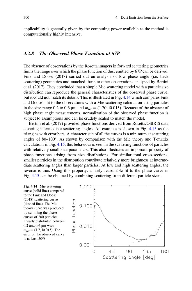
Fink and Doose (2018) carried out an analysis of low phase angle (i.e. back
scattering) geometries and matched these to other observations analysed by Bertini
et al. (2017). They concluded that a simple Mie scattering model with a particle size
distribution can reproduce the general characteristics of the observed phase curve,
but it could not match its details. This is illustrated in Fig. 4.14 which compares Fink
and Doose’s fit to the observations with a Mie scattering calculation using particles
in the size range 0.2 to 0.6 μm and m ref ¼ (1.70, i0.015). Because of the absence of
high phase angle measurements, normalization of the observed phase function is
subject to assumptions and can be crudely scaled to match the model.
Bertini et al. (2017) provided phase functions derived from Rosetta/OSIRIS data
covering intermediate scattering angles. An example is shown in Fig. 4.15 as the
triangles with error bars. A characteristic of all the curves is a minimum at scattering
angles of 80–100
. As shown by comparison with the Mie theory and T-matrix
calculations in Fig. 4.15, this behaviour is seen in the scattering functions of particles
with relatively small size parameters. This also illustrates an important property of
phase functions arising from size distributions. For similar total cross-sections,
smaller particles in the distribution contribute relatively more brightness at intermediate scattering angles than larger particles. At low and high scattering angles, the
reverse is true. Using this property, a fairly reasonable fit to the phase curve in
Fig. 4.15 can be obtained by combining scattering from different particle sizes.
Fig. 4.14 Mie scattering
curve (solid line) compared
to the Fink and Doose
(2018) scattering curve
(dashed line). The Mie
theory curve was produced
by summing the phase
curves of 200 particles
linearly distributed between
0.2 and 0.6 μm with
m ref ¼ (1.7, i0.015). The
error on the observed curve
is at least 50%
300
4 Dust Emission from the Surface
computationally highly intensive.
4.2.8 The Observed Phase Function at 67P
The absence of observations by the Rosetta imagers in forward scattering geometries
limits the range over which the phase function of dust emitted by 67P can be derived.
Fink and Doose (2018) carried out an analysis of low phase angle (i.e. back
scattering) geometries and matched these to other observations analysed by Bertini
et al. (2017). They concluded that a simple Mie scattering model with a particle size
distribution can reproduce the general characteristics of the observed phase curve,
but it could not match its details. This is illustrated in Fig. 4.14 which compares Fink
and Doose’s fit to the observations with a Mie scattering calculation using particles
in the size range 0.2 to 0.6 μm and m ref ¼ (1.70, i0.015). Because of the absence of
high phase angle measurements, normalization of the observed phase function is
subject to assumptions and can be crudely scaled to match the model.
Bertini et al. (2017) provided phase functions derived from Rosetta/OSIRIS data
covering intermediate scattering angles. An example is shown in Fig. 4.15 as the
triangles with error bars. A characteristic of all the curves is a minimum at scattering
angles of 80–100
. As shown by comparison with the Mie theory and T-matrix
calculations in Fig. 4.15, this behaviour is seen in the scattering functions of particles
with relatively small size parameters. This also illustrates an important property of
phase functions arising from size distributions. For similar total cross-sections,
smaller particles in the distribution contribute relatively more brightness at intermediate scattering angles than larger particles. At low and high scattering angles, the
reverse is true. Using this property, a fairly reasonable fit to the phase curve in
Fig. 4.15 can be obtained by combining scattering from different particle sizes.
Fig. 4.14 Mie scattering
curve (solid line) compared
to the Fink and Doose
(2018) scattering curve
(dashed line). The Mie
theory curve was produced
by summing the phase
curves of 200 particles
linearly distributed between
0.2 and 0.6 μm with
m ref ¼ (1.7, i0.015). The
error on the observed curve
is at least 50%
300
4 Dust Emission from the Surface