

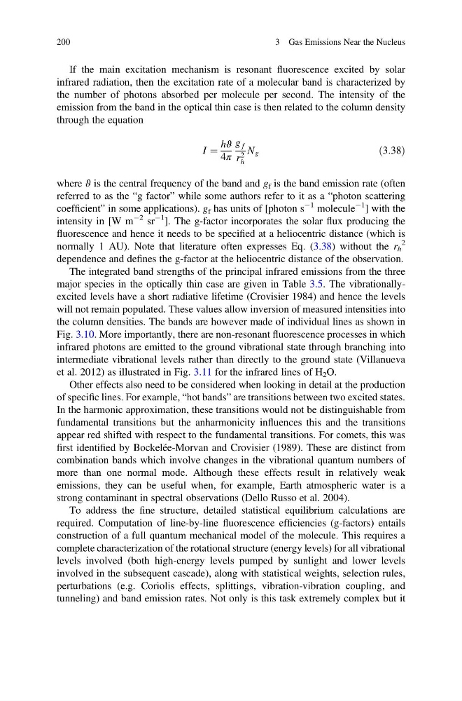
If the main excitation mechanism is resonant fluorescence excited by solar
infrared radiation, then the excitation rate of a molecular band is characterized by
the number of photons absorbed per molecule per second. The intensity of the
emission from the band in the optical thin case is then related to the column density
through the equation
I ¼
hϑ
4π
g f
r 2
h
N g
ð3:38Þ
where ϑ is the central frequency of the band and g f is the band emission rate (often
referred to as the “g factor” while some authors refer to it as a “photon scattering
coefficient” in some applications). g f has units of [photon s
À1 molecule
À1 ] with the
intensity in [W m
À2 sr
À1 ]. The g-factor incorporates the solar flux producing the
fluorescence and hence it needs to be specified at a heliocentric distance (which is
normally 1 AU). Note that literature often expresses Eq. (3.38) without the r h
2
dependence and defines the g-factor at the heliocentric distance of the observation.
The integrated band strengths of the principal infrared emissions from the three
major species in the optically thin case are given in Table 3.5. The vibrationallyexcited levels have a short radiative lifetime (Crovisier 1984) and hence the levels
will not remain populated. These values allow inversion of measured intensities into
the column densities. The bands are however made of individual lines as shown in
Fig. 3.10. More importantly, there are non-resonant fluorescence processes in which
infrared photons are emitted to the ground vibrational state through branching into
intermediate vibrational levels rather than directly to the ground state (Villanueva
et al. 2012) as illustrated in Fig. 3.11 for the infrared lines of H 2 O.
Other effects also need to be considered when looking in detail at the production
of specific lines. For example, “hot bands” are transitions between two excited states.
In the harmonic approximation, these transitions would not be distinguishable from
fundamental transitions but the anharmonicity influences this and the transitions
appear red shifted with respect to the fundamental transitions. For comets, this was
first identified by Bockelée-Morvan and Crovisier (1989). These are distinct from
combination bands which involve changes in the vibrational quantum numbers of
more than one normal mode. Although these effects result in relatively weak
emissions, they can be useful when, for example, Earth atmospheric water is a
strong contaminant in spectral observations (Dello Russo et al. 2004).
To address the fine structure, detailed statistical equilibrium calculations are
required. Computation of line-by-line fluorescence efficiencies (g-factors) entails
construction of a full quantum mechanical model of the molecule. This requires a
complete characterization of the rotational structure (energy levels) for all vibrational
levels involved (both high-energy levels pumped by sunlight and lower levels
involved in the subsequent cascade), along with statistical weights, selection rules,
perturbations (e.g. Coriolis effects, splittings, vibration-vibration coupling, and
tunneling) and band emission rates. Not only is this task extremely complex but it
200
3 Gas Emissions Near the Nucleus
infrared radiation, then the excitation rate of a molecular band is characterized by
the number of photons absorbed per molecule per second. The intensity of the
emission from the band in the optical thin case is then related to the column density
through the equation
I ¼
hϑ
4π
g f
r 2
h
N g
ð3:38Þ
where ϑ is the central frequency of the band and g f is the band emission rate (often
referred to as the “g factor” while some authors refer to it as a “photon scattering
coefficient” in some applications). g f has units of [photon s
À1 molecule
À1 ] with the
intensity in [W m
À2 sr
À1 ]. The g-factor incorporates the solar flux producing the
fluorescence and hence it needs to be specified at a heliocentric distance (which is
normally 1 AU). Note that literature often expresses Eq. (3.38) without the r h
2
dependence and defines the g-factor at the heliocentric distance of the observation.
The integrated band strengths of the principal infrared emissions from the three
major species in the optically thin case are given in Table 3.5. The vibrationallyexcited levels have a short radiative lifetime (Crovisier 1984) and hence the levels
will not remain populated. These values allow inversion of measured intensities into
the column densities. The bands are however made of individual lines as shown in
Fig. 3.10. More importantly, there are non-resonant fluorescence processes in which
infrared photons are emitted to the ground vibrational state through branching into
intermediate vibrational levels rather than directly to the ground state (Villanueva
et al. 2012) as illustrated in Fig. 3.11 for the infrared lines of H 2 O.
Other effects also need to be considered when looking in detail at the production
of specific lines. For example, “hot bands” are transitions between two excited states.
In the harmonic approximation, these transitions would not be distinguishable from
fundamental transitions but the anharmonicity influences this and the transitions
appear red shifted with respect to the fundamental transitions. For comets, this was
first identified by Bockelée-Morvan and Crovisier (1989). These are distinct from
combination bands which involve changes in the vibrational quantum numbers of
more than one normal mode. Although these effects result in relatively weak
emissions, they can be useful when, for example, Earth atmospheric water is a
strong contaminant in spectral observations (Dello Russo et al. 2004).
To address the fine structure, detailed statistical equilibrium calculations are
required. Computation of line-by-line fluorescence efficiencies (g-factors) entails
construction of a full quantum mechanical model of the molecule. This requires a
complete characterization of the rotational structure (energy levels) for all vibrational
levels involved (both high-energy levels pumped by sunlight and lower levels
involved in the subsequent cascade), along with statistical weights, selection rules,
perturbations (e.g. Coriolis effects, splittings, vibration-vibration coupling, and
tunneling) and band emission rates. Not only is this task extremely complex but it
200
3 Gas Emissions Near the Nucleus