

still has some limitations. Information for most hot bands for example, is not
available in community spectral databases (Villanueva et al. 2012).
To illustrate the influence on the infrared fine structure, we can use an on-line
resource called the Planetary Spectrum Generator (PSG)
3 which is now available to
support analyses (Villanueva et al. 2018). This is a radiative transfer suite allowing
synthesis of spectra for a broad range of planetary targets given appropriate input.
The tool has a specific template for 67P, allowing the generation of synthetic spectra
in the 0.1 μm–100 mm wavelength range. Figure 3.12 shows the result of a
calculation for a weak comet so that the optical depth is zero. Two different
temperatures for the gas are shown. Comparing this with Fig. 3.10, it can be seen
that the structure of the lines is appreciably different if non-LTE has to be assumed.
Figure 3.13 uses PSG to model VIRTIS-H point spectrometer observations of
67P at a time when optical thickness effects could be neglected. The plot shows the
sum of 21 observations were acquired between 24 Dec 2014 and 25 Jan 2015
(cf Bockelée-Morvan et al. 2015) with the spacecraft pointing off the limb. The
effective resolution of the instrument at this wavelength was around 3.3 nm and the
model calculation has been degraded to this resolution for comparison. Rosetta was
between 2.5 and 2.7 AU from the Sun at this time (pre-perihelion) with the column
density such that almost all the individual lines could be assumed to be optically thin
(see Fig. 3.15 later). The online model agrees fairly well with the data giving a
similar result to that seen in Bockelée-Morvan et al. (2015).
Collisional excitation is another primary means of excitation. The colliding
species may be electrons, ions (although their densities in the innermost coma are
far below that of neutrals) or other molecules (primarily H 2 O although CO may be of
relevance at larger heliocentric distances or in CO-rich comae).
An example of electron collision excitation is given in Fig. 3.14 which shows the
cross-section for excitation of the water molecule from the rotational ground-state to
the J ¼ 1 level (Itikawa and Mason 2005) and is from the Quantemol database
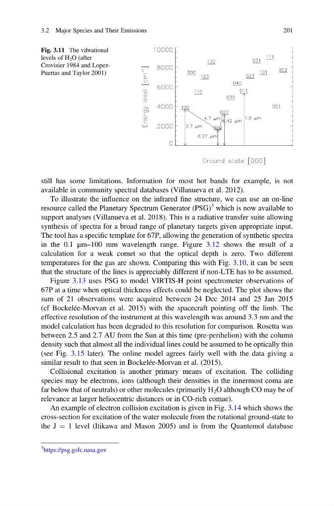
Fig. 3.11 The vibrational
levels of H 2 O (after
Crovisier 1984 and LopezPuertas and Taylor 2001)
3 https://psg.gsfc.nasa.gov
3.2 Major Species and Their Emissions
201
available in community spectral databases (Villanueva et al. 2012).
To illustrate the influence on the infrared fine structure, we can use an on-line
resource called the Planetary Spectrum Generator (PSG)
3 which is now available to
support analyses (Villanueva et al. 2018). This is a radiative transfer suite allowing
synthesis of spectra for a broad range of planetary targets given appropriate input.
The tool has a specific template for 67P, allowing the generation of synthetic spectra
in the 0.1 μm–100 mm wavelength range. Figure 3.12 shows the result of a
calculation for a weak comet so that the optical depth is zero. Two different
temperatures for the gas are shown. Comparing this with Fig. 3.10, it can be seen
that the structure of the lines is appreciably different if non-LTE has to be assumed.
Figure 3.13 uses PSG to model VIRTIS-H point spectrometer observations of
67P at a time when optical thickness effects could be neglected. The plot shows the
sum of 21 observations were acquired between 24 Dec 2014 and 25 Jan 2015
(cf Bockelée-Morvan et al. 2015) with the spacecraft pointing off the limb. The
effective resolution of the instrument at this wavelength was around 3.3 nm and the
model calculation has been degraded to this resolution for comparison. Rosetta was
between 2.5 and 2.7 AU from the Sun at this time (pre-perihelion) with the column
density such that almost all the individual lines could be assumed to be optically thin
(see Fig. 3.15 later). The online model agrees fairly well with the data giving a
similar result to that seen in Bockelée-Morvan et al. (2015).
Collisional excitation is another primary means of excitation. The colliding
species may be electrons, ions (although their densities in the innermost coma are
far below that of neutrals) or other molecules (primarily H 2 O although CO may be of
relevance at larger heliocentric distances or in CO-rich comae).
An example of electron collision excitation is given in Fig. 3.14 which shows the
cross-section for excitation of the water molecule from the rotational ground-state to
the J ¼ 1 level (Itikawa and Mason 2005) and is from the Quantemol database
Fig. 3.11 The vibrational
levels of H 2 O (after
Crovisier 1984 and LopezPuertas and Taylor 2001)
3 https://psg.gsfc.nasa.gov
3.2 Major Species and Their Emissions
201