

2. A low density, hot gas seen against a cooler background emits an emission line
spectrum.
3. A low density, cool gas in front of a hotter source of a continuous spectrum
creates an absorption spectrum.
This is illustrated in Fig. 3.3 with some data acquired on 4 November 2014 by the
MIRO experiment. The observation was relatively early in the mission with the
comet at a fairly high heliocentric distance and a low water production rate (~2 kg
s
À1 ). The sub-mm line of the main isotopologue of water vapour was therefore not
optically thick. The lower line in the plot shows water vapour (H 2
16 O) in emission
and corresponds to the second of Kirchhoff’s laws—a relatively warm gas viewed
against a colder background. The upper line shows the same line but now in
absorption corresponding to the third of Kirchhoff’s laws—a relative cold gas
viewed against the warmer background of the nucleus. The nucleus here was not
very warm because it was being viewed from a phase angle of 114
, i.e. the
sub-spacecraft point was above the nightside. However it was sufficiently warm to
show the rapidly cooling gas in absorption.
Another point of note in Fig. 3.3 is the Doppler shift between the two lines. The
observation towards to the nucleus shows a negative Doppler shift of the line—the
gas being observed is mostly moving towards the instrument along the line of sight.
Looking off the limb, however, we see that much of the gas is moving away from the
observer. This is qualitatively consistent with most of the gas emission being
towards the Sun with the observer being at a phase angle of 114
.
As the gas production rate increases, observations of H 2
16 O close to the nucleus
become increasing susceptible to optical depth effects. We illustrate this with a
model calculation using Eq. (3.20) and the output from a gas dynamics simulation.
The latter provides the H 2 O density, rotational temperature and line-of-sight gas
velocity as input (Fig. 3.4) for the radiative transfer model. A 110 K nucleus
background has been assumed. The results (Fig. 3.5) show the effect of opacity on
the H 2
16 O line and the appearance of the H 2
18 O line which is not saturated. The
model here assumes LTE in which the source function is given by the Planck
function.
Under the assumption of LTE, we can now attempt to fit MIRO data. An example
of two fits to an observation from near the time of perihelion (10 July 2015) is given
in Fig. 3.6. The self-absorption of the H 2
16 O line is evident in the centre panel. The
H 2
18
O line is seen in the lower panel and is not saturated. The dashed lines were
computed with a surface temperature model based on Eq. (2.101). The models
suggest that the velocity of the gas is not high enough. For the dot-dashed lines,
the surface temperature has been increased proportional to the cosine of the solar
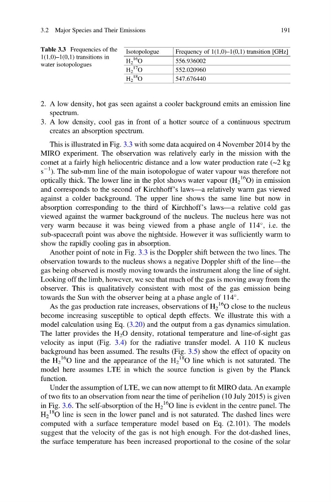
Table 3.3 Frequencies of the
1(1,0)–1(0,1) transitions in
water isotopologues
Isotopologue
Frequency of 1(1,0)–1(0,1) transition [GHz]
H 2
16
O
556.936002
H 2
17
O
552.020960
H 2
18
O
547.676440
3.2 Major Species and Their Emissions
191
spectrum.
3. A low density, cool gas in front of a hotter source of a continuous spectrum
creates an absorption spectrum.
This is illustrated in Fig. 3.3 with some data acquired on 4 November 2014 by the
MIRO experiment. The observation was relatively early in the mission with the
comet at a fairly high heliocentric distance and a low water production rate (~2 kg
s
À1 ). The sub-mm line of the main isotopologue of water vapour was therefore not
optically thick. The lower line in the plot shows water vapour (H 2
16 O) in emission
and corresponds to the second of Kirchhoff’s laws—a relatively warm gas viewed
against a colder background. The upper line shows the same line but now in
absorption corresponding to the third of Kirchhoff’s laws—a relative cold gas
viewed against the warmer background of the nucleus. The nucleus here was not
very warm because it was being viewed from a phase angle of 114
, i.e. the
sub-spacecraft point was above the nightside. However it was sufficiently warm to
show the rapidly cooling gas in absorption.
Another point of note in Fig. 3.3 is the Doppler shift between the two lines. The
observation towards to the nucleus shows a negative Doppler shift of the line—the
gas being observed is mostly moving towards the instrument along the line of sight.
Looking off the limb, however, we see that much of the gas is moving away from the
observer. This is qualitatively consistent with most of the gas emission being
towards the Sun with the observer being at a phase angle of 114
.
As the gas production rate increases, observations of H 2
16 O close to the nucleus
become increasing susceptible to optical depth effects. We illustrate this with a
model calculation using Eq. (3.20) and the output from a gas dynamics simulation.
The latter provides the H 2 O density, rotational temperature and line-of-sight gas
velocity as input (Fig. 3.4) for the radiative transfer model. A 110 K nucleus
background has been assumed. The results (Fig. 3.5) show the effect of opacity on
the H 2
16 O line and the appearance of the H 2
18 O line which is not saturated. The
model here assumes LTE in which the source function is given by the Planck
function.
Under the assumption of LTE, we can now attempt to fit MIRO data. An example
of two fits to an observation from near the time of perihelion (10 July 2015) is given
in Fig. 3.6. The self-absorption of the H 2
16 O line is evident in the centre panel. The
H 2
18
O line is seen in the lower panel and is not saturated. The dashed lines were
computed with a surface temperature model based on Eq. (2.101). The models
suggest that the velocity of the gas is not high enough. For the dot-dashed lines,
the surface temperature has been increased proportional to the cosine of the solar
Table 3.3 Frequencies of the
1(1,0)–1(0,1) transitions in
water isotopologues
Isotopologue
Frequency of 1(1,0)–1(0,1) transition [GHz]
H 2
16
O
556.936002
H 2
17
O
552.020960
H 2
18
O
547.676440
3.2 Major Species and Their Emissions
191