

Deep Impact spacecraft that the thermal inertia was <250 TIU for 103P/Hartley 2
and <45 TIU for 9P/Tempel 1. For both comets, the temperature of the regions with
exposed water ice was more than 100 K above the sublimation temperature of water
ice indicating that the thermal emission was dominated by dust. Furthermore, the
water ice could not be intimately mixed with dust at the scale of observations.
Similar results can be obtained for the nucleus of 67P. We can illustrate this using
the MIRO measurements of the brightness temperature of the continuum thermal
emission. This was measured at two frequencies (188.2 GHz and 562.8 GHz). These
measurements do not give the temperature at the actual surface. It is often assumed
that the two frequencies sample two discrete depths below the surface but although
this is good approximation it is not completely accurate. The effective temperature,
T eff , is computed by integrating the thermal emission contribution of each sublayer
below the surface, weighted by a radiative transfer function, which expresses the
extinction of the thermal emission as it propagates towards the surface. T eff , assuming a scatter-free homogeneous layer under conditions of local thermodynamic
equilibrium, is determined by
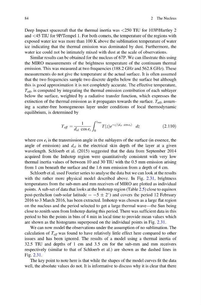
T eff ¼
1
d el cos e t
Z z max
0
T z
ð Þe
Àz= d el cos e t
ð
Þ dz
ð2:110Þ
where cos e t is the transmission angle in the sublayers of the surface (in essence, the
angle of emission) and d el is the electrical skin depth of the layer at a given
wavelength. Schloerb et al. (2015) suggested that the data from September 2014
acquired from the Imhotep region were quantitatively consistent with very low
thermal inertia values of between 10 and 30 TIU with the 0.5 mm emission arising
from 1 cm beneath the surface and the 1.6 mm emission from a depth of 4 cm.
Schloerb et al. used Fourier series to analyse the data but we can look at the results
with the rather more physical model described above. In Fig. 2.31, brightness
temperatures from the sub-mm and mm receivers of MIRO are plotted as individual
points. A sub-set of data that looks at the Imhotep region (Table 2.5) close to equinox
post-perihelion (sub-solar latitude ¼ À5 Æ 2
) and covers the period 12 February
2016 to 3 March 2016, has been extracted. Imhotep was chosen as a large flat region
on the nucleus and the period selected to get a large thermal wave—the Sun being
close to zenith seen from Imhotep during this period. There was sufficient data in this
period to bin the points in bins of 4 min in local time to provide mean values which
are shown as the histograms superposed on the individual points in Fig. 2.31.
We can now model the observations under the assumption of no sublimation. The
calculation of T eff was found to have relatively little effect here compared to other
issues and has been ignored. The results of a model using a thermal inertia of
32.5 TIU and depths of 1 cm and 3.5 cm for the sub-mm and mm receivers
respectively (similar to that of Schloerb et al.) are shown as the dashed lines in
Fig. 2.31.
The key point to note here is that while the shapes of the model curves fit the data
well, the absolute values do not. It is informative to discuss why it is clear that there
84
2 The Nucleus
and <45 TIU for 9P/Tempel 1. For both comets, the temperature of the regions with
exposed water ice was more than 100 K above the sublimation temperature of water
ice indicating that the thermal emission was dominated by dust. Furthermore, the
water ice could not be intimately mixed with dust at the scale of observations.
Similar results can be obtained for the nucleus of 67P. We can illustrate this using
the MIRO measurements of the brightness temperature of the continuum thermal
emission. This was measured at two frequencies (188.2 GHz and 562.8 GHz). These
measurements do not give the temperature at the actual surface. It is often assumed
that the two frequencies sample two discrete depths below the surface but although
this is good approximation it is not completely accurate. The effective temperature,
T eff , is computed by integrating the thermal emission contribution of each sublayer
below the surface, weighted by a radiative transfer function, which expresses the
extinction of the thermal emission as it propagates towards the surface. T eff , assuming a scatter-free homogeneous layer under conditions of local thermodynamic
equilibrium, is determined by
T eff ¼
1
d el cos e t
Z z max
0
T z
ð Þe
Àz= d el cos e t
ð
Þ dz
ð2:110Þ
where cos e t is the transmission angle in the sublayers of the surface (in essence, the
angle of emission) and d el is the electrical skin depth of the layer at a given
wavelength. Schloerb et al. (2015) suggested that the data from September 2014
acquired from the Imhotep region were quantitatively consistent with very low
thermal inertia values of between 10 and 30 TIU with the 0.5 mm emission arising
from 1 cm beneath the surface and the 1.6 mm emission from a depth of 4 cm.
Schloerb et al. used Fourier series to analyse the data but we can look at the results
with the rather more physical model described above. In Fig. 2.31, brightness
temperatures from the sub-mm and mm receivers of MIRO are plotted as individual
points. A sub-set of data that looks at the Imhotep region (Table 2.5) close to equinox
post-perihelion (sub-solar latitude ¼ À5 Æ 2
) and covers the period 12 February
2016 to 3 March 2016, has been extracted. Imhotep was chosen as a large flat region
on the nucleus and the period selected to get a large thermal wave—the Sun being
close to zenith seen from Imhotep during this period. There was sufficient data in this
period to bin the points in bins of 4 min in local time to provide mean values which
are shown as the histograms superposed on the individual points in Fig. 2.31.
We can now model the observations under the assumption of no sublimation. The
calculation of T eff was found to have relatively little effect here compared to other
issues and has been ignored. The results of a model using a thermal inertia of
32.5 TIU and depths of 1 cm and 3.5 cm for the sub-mm and mm receivers
respectively (similar to that of Schloerb et al.) are shown as the dashed lines in
Fig. 2.31.
The key point to note here is that while the shapes of the model curves fit the data
well, the absolute values do not. It is informative to discuss why it is clear that there
84
2 The Nucleus