

6 The Discovery of the Higgs Boson at the LHC
293
The H → τ τ mode is studied via tau decays to eμ, μμ, eτ h , μτ h , τ h τ h ,
where electrons and muons arise from leptonic τ -decays and τ h denotes a τ
lepton decaying hadronically. Each of these categories is further divided into three
sub-categories labeled 0-jet, boosted and VBF. The 0-jet category helps constrain
background normalisation, identification efficiencies, and energy scales, and systematic uncertainties in the background model. The main irreducible background,
Z → τ τ production, and the largest reducible backgrounds (W + jets, QCD multijet
production, and top quark pair) are evaluated from control samples in data.
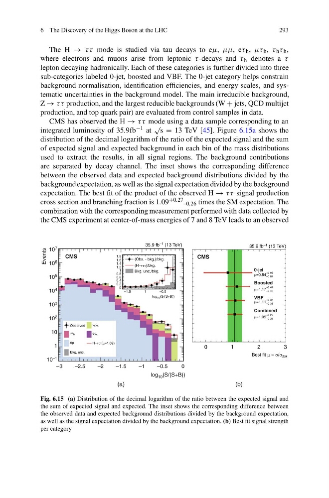
CMS has observed the H → τ τ mode using a data sample corresponding to an
integrated luminosity of 35.9fb −1 at
√
s = 13 TeV [45]. Figure 6.15a shows the
distribution of the decimal logarithm of the ratio of the expected signal and the sum
of expected signal and expected background in each bin of the mass distributions
used to extract the results, in all signal regions. The background contributions
are separated by decay channel. The inset shows the corresponding difference
between the observed data and expected background distributions divided by the
background expectation, as well as the signal expectation divided by the background
expectation. The best fit of the product of the observed H → τ τ signal production
cross section and branching fraction is 1.09 +0.27 –0.26 times the SM expectation. The
combination with the corresponding measurement performed with data collected by
the CMS experiment at center-of-mass energies of 7 and 8 TeV leads to an observed
CMS
CMS
10 6
1.6
1.4
1.2
1
0.8
0.6
0.4
0.2
1.8
0
1
(Obs. - bkg.)/bkg.
0-jet
=0.84
+0.89
–0.89
Boosted
=1.17
+0.47
–0.40
VBF
=1.11
+0.34
–0.35
Combined
Best fit = / SM
=1.09
+0.27
–0.26
(H
)/bkg.
H
( =1.09)
e h
e
h
h h
Bkg. unc./bkg.
Bkg. unc.
Observed
–1.5
–0.5
10 5
10 4
10 3
10 2
10
1
10 7
Events
10 –1
–0.5
log 10 (S/(S+B))
log 10 (S/(S+B))
–1
–1.5
(a)
(b)
–2
–2.5
–3
2
0
1
3
0
35.9 fb –1 (13 TeV)
35.9 fb –1 (13 TeV)
Fig. 6.15 (a) Distribution of the decimal logarithm of the ratio between the expected signal and
the sum of expected signal and expected. The inset shows the corresponding difference between
the observed data and expected background distributions divided by the background expectation,
as well as the signal expectation divided by the background expectation. (b) Best fit signal strength
per category
293
The H → τ τ mode is studied via tau decays to eμ, μμ, eτ h , μτ h , τ h τ h ,
where electrons and muons arise from leptonic τ -decays and τ h denotes a τ
lepton decaying hadronically. Each of these categories is further divided into three
sub-categories labeled 0-jet, boosted and VBF. The 0-jet category helps constrain
background normalisation, identification efficiencies, and energy scales, and systematic uncertainties in the background model. The main irreducible background,
Z → τ τ production, and the largest reducible backgrounds (W + jets, QCD multijet
production, and top quark pair) are evaluated from control samples in data.
CMS has observed the H → τ τ mode using a data sample corresponding to an
integrated luminosity of 35.9fb −1 at
√
s = 13 TeV [45]. Figure 6.15a shows the
distribution of the decimal logarithm of the ratio of the expected signal and the sum
of expected signal and expected background in each bin of the mass distributions
used to extract the results, in all signal regions. The background contributions
are separated by decay channel. The inset shows the corresponding difference
between the observed data and expected background distributions divided by the
background expectation, as well as the signal expectation divided by the background
expectation. The best fit of the product of the observed H → τ τ signal production
cross section and branching fraction is 1.09 +0.27 –0.26 times the SM expectation. The
combination with the corresponding measurement performed with data collected by
the CMS experiment at center-of-mass energies of 7 and 8 TeV leads to an observed
CMS
CMS
10 6
1.6
1.4
1.2
1
0.8
0.6
0.4
0.2
1.8
0
1
(Obs. - bkg.)/bkg.
0-jet
=0.84
+0.89
–0.89
Boosted
=1.17
+0.47
–0.40
VBF
=1.11
+0.34
–0.35
Combined
Best fit = / SM
=1.09
+0.27
–0.26
(H
)/bkg.
H
( =1.09)
e h
e
h
h h
Bkg. unc./bkg.
Bkg. unc.
Observed
–1.5
–0.5
10 5
10 4
10 3
10 2
10
1
10 7
Events
10 –1
–0.5
log 10 (S/(S+B))
log 10 (S/(S+B))
–1
–1.5
(a)
(b)
–2
–2.5
–3
2
0
1
3
0
35.9 fb –1 (13 TeV)
35.9 fb –1 (13 TeV)
Fig. 6.15 (a) Distribution of the decimal logarithm of the ratio between the expected signal and
the sum of expected signal and expected. The inset shows the corresponding difference between
the observed data and expected background distributions divided by the background expectation,
as well as the signal expectation divided by the background expectation. (b) Best fit signal strength
per category