

224
H. Wittig
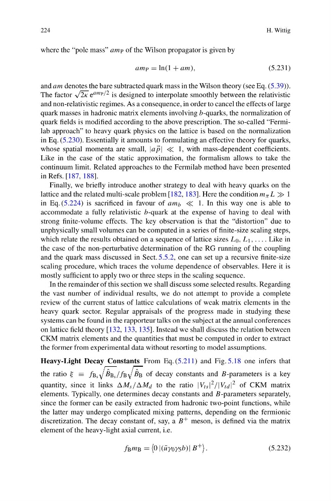
where the “pole mass” am P of the Wilson propagator is given by
am P = ln(1 + am),
(5.231)
and am denotes the bare subtracted quark mass in the Wilson theory (see Eq. (5.39)).
The factor
√
2κ e am P /2 is designed to interpolate smoothly between the relativistic
and non-relativistic regimes. As a consequence, in order to cancel the effects of large
quark masses in hadronic matrix elements involving b-quarks, the normalization of
quark fields is modified according to the above prescription. The so-called “Fermilab approach” to heavy quark physics on the lattice is based on the normalization
in Eq. (5.230). Essentially it amounts to formulating an effective theory for quarks,
whose spatial momenta are small, |a
p| | 1, with mass-dependent coefficients.
Like in the case of the static approximation, the formalism allows to take the
continuum limit. Related approaches to the Fermilab method have been presented
in Refs. [187, 188].
Finally, we briefly introduce another strategy to deal with heavy quarks on the
lattice and the related multi-scale problem [182, 183]. Here the condition m π L 1
in Eq. (5.224) is sacrificed in favour of am b 1. In this way one is able to
accommodate a fully relativistic b-quark at the expense of having to deal with
strong finite-volume effects. The key observation is that the “distortion” due to
unphysically small volumes can be computed in a series of finite-size scaling steps,
which relate the results obtained on a sequence of lattice sizes L 0 , L 1 , . . . . Like in
the case of the non-perturbative determination of the RG running of the coupling
and the quark mass discussed in Sect. 5.5.2, one can set up a recursive finite-size
scaling procedure, which traces the volume dependence of observables. Here it is
mostly sufficient to apply two or three steps in the scaling sequence.
In the remainder of this section we shall discuss some selected results. Regarding
the vast number of individual results, we do not attempt to provide a complete
review of the current status of lattice calculations of weak matrix elements in the
heavy quark sector. Regular appraisals of the progress made in studying these
systems can be found in the rapporteur talks on the subject at the annual conferences
on lattice field theory [132, 133, 135]. Instead we shall discuss the relation between
CKM matrix elements and the quantities that must be computed in order to extract
the former from experimental data without resorting to model assumptions.
Heavy-Light Decay Constants From Eq. (5.211) and Fig. 5.18 one infers that
the ratio ξ ≡ f B s
ˆ
B B s /f B
ˆ
B B of decay constants and B-parameters is a key
quantity, since it links s //M d to the ratio |V ts | 2 /|V td | 2 of CKM matrix
elements. Typically, one determines decay constants and B-parameters separately,
since the former can be easily extracted from hadronic two-point functions, while
the latter may undergo complicated mixing patterns, depending on the fermionic
discretization. The decay constant of, say, a B + meson, is defined via the matrix
element of the heavy-light axial current, i.e.
f B m B =
0 |( ¯
uγ 0 γ 5 b)| B
+
.
(5.232)
H. Wittig
where the “pole mass” am P of the Wilson propagator is given by
am P = ln(1 + am),
(5.231)
and am denotes the bare subtracted quark mass in the Wilson theory (see Eq. (5.39)).
The factor
√
2κ e am P /2 is designed to interpolate smoothly between the relativistic
and non-relativistic regimes. As a consequence, in order to cancel the effects of large
quark masses in hadronic matrix elements involving b-quarks, the normalization of
quark fields is modified according to the above prescription. The so-called “Fermilab approach” to heavy quark physics on the lattice is based on the normalization
in Eq. (5.230). Essentially it amounts to formulating an effective theory for quarks,
whose spatial momenta are small, |a
p| | 1, with mass-dependent coefficients.
Like in the case of the static approximation, the formalism allows to take the
continuum limit. Related approaches to the Fermilab method have been presented
in Refs. [187, 188].
Finally, we briefly introduce another strategy to deal with heavy quarks on the
lattice and the related multi-scale problem [182, 183]. Here the condition m π L 1
in Eq. (5.224) is sacrificed in favour of am b 1. In this way one is able to
accommodate a fully relativistic b-quark at the expense of having to deal with
strong finite-volume effects. The key observation is that the “distortion” due to
unphysically small volumes can be computed in a series of finite-size scaling steps,
which relate the results obtained on a sequence of lattice sizes L 0 , L 1 , . . . . Like in
the case of the non-perturbative determination of the RG running of the coupling
and the quark mass discussed in Sect. 5.5.2, one can set up a recursive finite-size
scaling procedure, which traces the volume dependence of observables. Here it is
mostly sufficient to apply two or three steps in the scaling sequence.
In the remainder of this section we shall discuss some selected results. Regarding
the vast number of individual results, we do not attempt to provide a complete
review of the current status of lattice calculations of weak matrix elements in the
heavy quark sector. Regular appraisals of the progress made in studying these
systems can be found in the rapporteur talks on the subject at the annual conferences
on lattice field theory [132, 133, 135]. Instead we shall discuss the relation between
CKM matrix elements and the quantities that must be computed in order to extract
the former from experimental data without resorting to model assumptions.
Heavy-Light Decay Constants From Eq. (5.211) and Fig. 5.18 one infers that
the ratio ξ ≡ f B s
ˆ
B B s /f B
ˆ
B B of decay constants and B-parameters is a key
quantity, since it links s //M d to the ratio |V ts | 2 /|V td | 2 of CKM matrix
elements. Typically, one determines decay constants and B-parameters separately,
since the former can be easily extracted from hadronic two-point functions, while
the latter may undergo complicated mixing patterns, depending on the fermionic
discretization. The decay constant of, say, a B + meson, is defined via the matrix
element of the heavy-light axial current, i.e.
f B m B =
0 |( ¯
uγ 0 γ 5 b)| B
+
.
(5.232)