

5 QCD on the Lattice
161
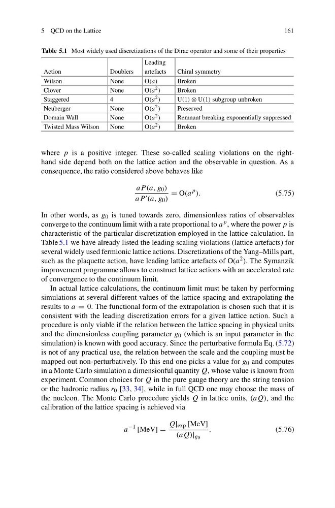
Table 5.1 Most widely used discretizations of the Dirac operator and some of their properties
Leading
Action
Doublers
artefacts
Chiral symmetry
Wilson
None
O(a)
Broken
Clover
None
O(a 2 )
Broken
Staggered
4
O(a 2 )
U(1) ⊗ U(1) subgroup unbroken
Neuberger
None
O(a 2 )
Preserved
Domain Wall
None
O(a 2 )
Remnant breaking exponentially suppressed
Twisted Mass Wilson
None
O(a 2 )
Broken
where p is a positive integer. These so-called scaling violations on the righthand side depend both on the lattice action and the observable in question. As a
consequence, the ratio considered above behaves like
aP (a, g 0 )
aP (a, g 0 )
= O(a
p ).
(5.75)
In other words, as g 0 is tuned towards zero, dimensionless ratios of observables
converge to the continuum limit with a rate proportional to a p , where the power p is
characteristic of the particular discretization employed in the lattice calculation. In
Table 5.1 we have already listed the leading scaling violations (lattice artefacts) for
several widely used fermionic lattice actions. Discretizations of the Yang–Mills part,
such as the plaquette action, have leading lattice artefacts of O(a 2 ). The Symanzik
improvement programme allows to construct lattice actions with an accelerated rate
of convergence to the continuum limit.
In actual lattice calculations, the continuum limit must be taken by performing
simulations at several different values of the lattice spacing and extrapolating the
results to a = 0. The functional form of the extrapolation is chosen such that it is
consistent with the leading discretization errors for a given lattice action. Such a
procedure is only viable if the relation between the lattice spacing in physical units
and the dimensionless coupling parameter g 0 (which is an input parameter in the
simulation) is known with good accuracy. Since the perturbative formula Eq. (5.72)
is not of any practical use, the relation between the scale and the coupling must be
mapped out non-perturbatively. To this end one picks a value for g 0 and computes
in a Monte Carlo simulation a dimensionful quantity Q, whose value is known from
experiment. Common choices for Q in the pure gauge theory are the string tension
or the hadronic radius r 0 [33, 34], while in full QCD one may choose the mass of
the nucleon. The Monte Carlo procedure yields Q in lattice units, (aQ), and the
calibration of the lattice spacing is achieved via
a
−1
[MeV] =
Q| exp [MeV]
(aQ)| g 0
.
(5.76)
161
Table 5.1 Most widely used discretizations of the Dirac operator and some of their properties
Leading
Action
Doublers
artefacts
Chiral symmetry
Wilson
None
O(a)
Broken
Clover
None
O(a 2 )
Broken
Staggered
4
O(a 2 )
U(1) ⊗ U(1) subgroup unbroken
Neuberger
None
O(a 2 )
Preserved
Domain Wall
None
O(a 2 )
Remnant breaking exponentially suppressed
Twisted Mass Wilson
None
O(a 2 )
Broken
where p is a positive integer. These so-called scaling violations on the righthand side depend both on the lattice action and the observable in question. As a
consequence, the ratio considered above behaves like
aP (a, g 0 )
aP (a, g 0 )
= O(a
p ).
(5.75)
In other words, as g 0 is tuned towards zero, dimensionless ratios of observables
converge to the continuum limit with a rate proportional to a p , where the power p is
characteristic of the particular discretization employed in the lattice calculation. In
Table 5.1 we have already listed the leading scaling violations (lattice artefacts) for
several widely used fermionic lattice actions. Discretizations of the Yang–Mills part,
such as the plaquette action, have leading lattice artefacts of O(a 2 ). The Symanzik
improvement programme allows to construct lattice actions with an accelerated rate
of convergence to the continuum limit.
In actual lattice calculations, the continuum limit must be taken by performing
simulations at several different values of the lattice spacing and extrapolating the
results to a = 0. The functional form of the extrapolation is chosen such that it is
consistent with the leading discretization errors for a given lattice action. Such a
procedure is only viable if the relation between the lattice spacing in physical units
and the dimensionless coupling parameter g 0 (which is an input parameter in the
simulation) is known with good accuracy. Since the perturbative formula Eq. (5.72)
is not of any practical use, the relation between the scale and the coupling must be
mapped out non-perturbatively. To this end one picks a value for g 0 and computes
in a Monte Carlo simulation a dimensionful quantity Q, whose value is known from
experiment. Common choices for Q in the pure gauge theory are the string tension
or the hadronic radius r 0 [33, 34], while in full QCD one may choose the mass of
the nucleon. The Monte Carlo procedure yields Q in lattice units, (aQ), and the
calibration of the lattice spacing is achieved via
a
−1
[MeV] =
Q| exp [MeV]
(aQ)| g 0
.
(5.76)