

4 QCD: The Theory of Strong Interactions
105
in α s (Q) we decide to choose α s (Q/2) the coefficients c 2 and c 3 change. In the MS
scheme, for γ -exchange and n f = 5, which are good approximations for 2m b <<
Q << m Z , one has:
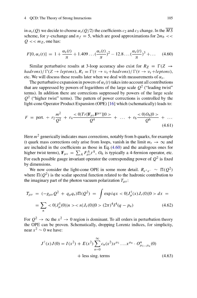
F [0, α s (t)] = 1 +
α s (t)
π
+ 1.409 . . . (
α s (t)
π
)
2
− 12.8 . . . (
α s (t)
π
)
3
+. . . (4.60)
Similar perturbative results at 3-loop accuracy also exist for R Z = (Z →
hadrons)/ /(Z → leptons), R τ = (τ → ν τ +hadrons)/ /(τ → ν τ +leptons),
etc. We will discuss these results later when we deal with measurements of α s .
The perturbative expansion in powers of α s (t) takes into account all contributions
that are suppressed by powers of logarithms of the large scale Q 2 (“leading twist”
terms). In addition there are corrections suppressed by powers of the large scale
Q 2 (“higher twist” terms). The pattern of power corrections is controlled by the
light-cone Operator Product Expansion (OPE) [16] which (schematically) leads to:
F = pert. + r 2
m 2
Q 2 + r 4
< 0|T r[F μν F μν ]|0 >
Q 4
+ . . . + r 6
< 0|O 6 |0 >
Q 6
+ . . .
(4.61)
Here m 2 generically indicates mass corrections, notably from b quarks, for example
(t quark mass corrections only arise from loops, vanish in the limit m t → ∞ and
are included in the coefficients as those in Eq. (4.60) and the analogous ones for
higher twist terms), F μν =
A F A
μν t A , O 6 is typically a 4-fermion operator, etc.
For each possible gauge invariant operator the corresponding power of Q 2 is fixed
by dimensions.
We now consider the light-cone OPE in some more detail. R e + e − ∼ 2 )
where (Q 2 ) is the scalar spectral function related to the hadronic contribution to
the imaginary part of the photon vacuum polarization T μν :
T μν = (−g μν Q
2
+ q μ q ν ))(Q
2 ) =
exp iqx < 0|J
†
μ (x)J ν (0)|0 > dx =
=
n
< 0|J
†
μ (0)|n >< n|J ν (0)|0 > (2π)
4 δ
4 (q − p n )
(4.62)
For Q 2 → ∞ the x 2 → 0 region is dominant. To all orders in perturbation theory
the OPE can be proven. Schematically, dropping Lorentz indices, for simplicity,
near x 2 ∼ 0 we have:
J
† (x)J (0) = I (x
2 ) + E(x
2 )
∞
n=0
c n (x
2 )x
μ 1 . . . x
μ n · O
n
μ 1 ...μ n
(0)
+ less sing. terms
(4.63)
105
in α s (Q) we decide to choose α s (Q/2) the coefficients c 2 and c 3 change. In the MS
scheme, for γ -exchange and n f = 5, which are good approximations for 2m b <<
Q << m Z , one has:
F [0, α s (t)] = 1 +
α s (t)
π
+ 1.409 . . . (
α s (t)
π
)
2
− 12.8 . . . (
α s (t)
π
)
3
+. . . (4.60)
Similar perturbative results at 3-loop accuracy also exist for R Z = (Z →
hadrons)/ /(Z → leptons), R τ = (τ → ν τ +hadrons)/ /(τ → ν τ +leptons),
etc. We will discuss these results later when we deal with measurements of α s .
The perturbative expansion in powers of α s (t) takes into account all contributions
that are suppressed by powers of logarithms of the large scale Q 2 (“leading twist”
terms). In addition there are corrections suppressed by powers of the large scale
Q 2 (“higher twist” terms). The pattern of power corrections is controlled by the
light-cone Operator Product Expansion (OPE) [16] which (schematically) leads to:
F = pert. + r 2
m 2
Q 2 + r 4
< 0|T r[F μν F μν ]|0 >
Q 4
+ . . . + r 6
< 0|O 6 |0 >
Q 6
+ . . .
(4.61)
Here m 2 generically indicates mass corrections, notably from b quarks, for example
(t quark mass corrections only arise from loops, vanish in the limit m t → ∞ and
are included in the coefficients as those in Eq. (4.60) and the analogous ones for
higher twist terms), F μν =
A F A
μν t A , O 6 is typically a 4-fermion operator, etc.
For each possible gauge invariant operator the corresponding power of Q 2 is fixed
by dimensions.
We now consider the light-cone OPE in some more detail. R e + e − ∼ 2 )
where (Q 2 ) is the scalar spectral function related to the hadronic contribution to
the imaginary part of the photon vacuum polarization T μν :
T μν = (−g μν Q
2
+ q μ q ν ))(Q
2 ) =
exp iqx < 0|J
†
μ (x)J ν (0)|0 > dx =
=
n
< 0|J
†
μ (0)|n >< n|J ν (0)|0 > (2π)
4 δ
4 (q − p n )
(4.62)
For Q 2 → ∞ the x 2 → 0 region is dominant. To all orders in perturbation theory
the OPE can be proven. Schematically, dropping Lorentz indices, for simplicity,
near x 2 ∼ 0 we have:
J
† (x)J (0) = I (x
2 ) + E(x
2 )
∞
n=0
c n (x
2 )x
μ 1 . . . x
μ n · O
n
μ 1 ...μ n
(0)
+ less sing. terms
(4.63)