

13 Pattern Recognition and Reconstruction
589
with
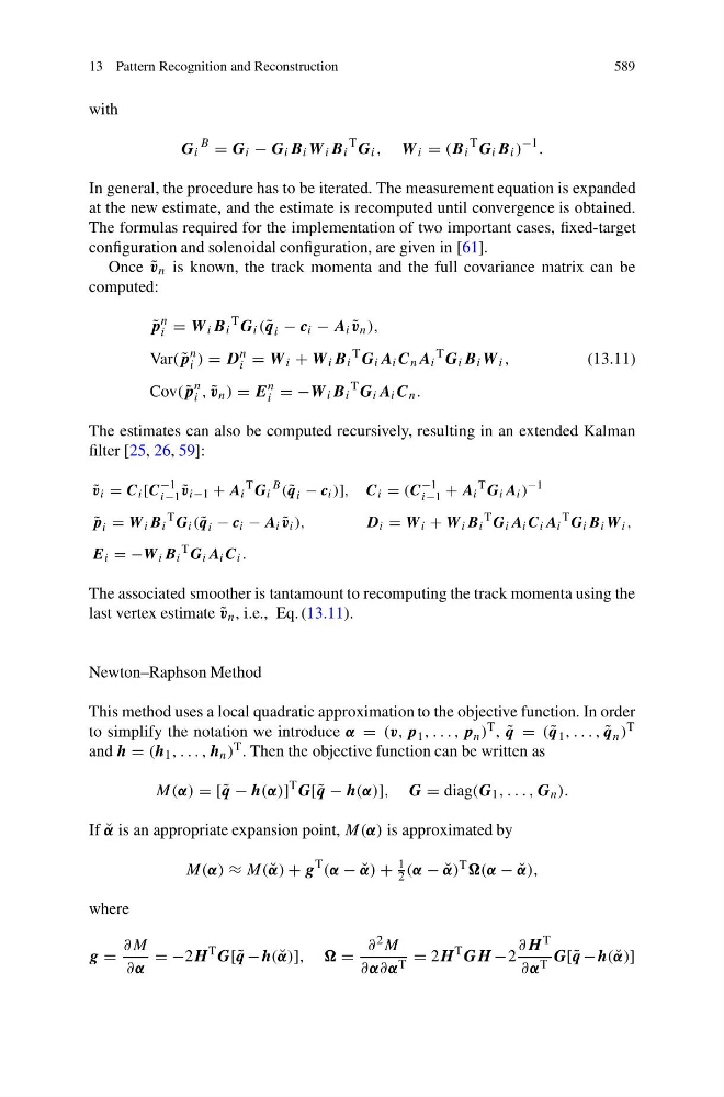
G i
B
= G i − G i B i W i B i
T G i , W i = (B i
T G i B i )
−1 .
In general, the procedure has to be iterated. The measurement equation is expanded
at the new estimate, and the estimate is recomputed until convergence is obtained.
The formulas required for the implementation of two important cases, fixed-target
configuration and solenoidal configuration, are given in [61].
Once ˜
v n is known, the track momenta and the full covariance matrix can be
computed:
˜
p
n
i = W i B i
T G i ( ˜
q i − c i − A i ˜
v n ),
Var( ˜
p
n
i ) = D
n
i = W i + W i B i
T G i A i C n A i
T G i B i W i ,
(13.11)
Cov( ˜
p
n
i , ˜
v n ) = E
n
i = −W i B i
T G i A i C n .
The estimates can also be computed recursively, resulting in an extended Kalman
filter [25, 26, 59]:
˜
v i = C i [C
−1
i−1 ˜
v i−1 + A i
T G i
B ( ˜
q i − c i )], C i = (C
−1
i−1 + A i
T G i A i )
−1
˜
p i = W i B i
T G i ( ˜
q i − c i − A i ˜
v i ),
D i = W i + W i B i
T G i A i C i A i
T G i B i W i ,
E i = −W i B i
T G i A i C i .
The associated smoother is tantamount to recomputing the track momenta using the
last vertex estimate ˜
v n , i.e., Eq. (13.11).
Newton–Raphson Method
This method uses a local quadratic approximation to the objective function. In order
to simplify the notation we introduce α = (v, p 1 , . . . , p n ) T , ˜
q = ( ˜
q 1 , . . . , ˜
q n ) T
and h = (h 1 , . . . , h n ) T . Then the objective function can be written as
M(α) = [˜ q − h(α)]
T G[ ˜
q − h(α)], G = diag(G 1 , . . . , G n ).
If ˘
α is an appropriate expansion point, M(α) is approximated by
M(α) ≈ M( ˘
α) + g
T (α − ˘
α) +
1
2 (α − ˘
α) T − ˘
α),
where
g =
∂M
∂α
= −2H
T G[ ˜
q −h( ˘
α)], =
∂ 2 M
∂α∂α T = 2H
T GH −2
∂H T
∂α T G[ ˜
q −h( ˘
α)]
589
with
G i
B
= G i − G i B i W i B i
T G i , W i = (B i
T G i B i )
−1 .
In general, the procedure has to be iterated. The measurement equation is expanded
at the new estimate, and the estimate is recomputed until convergence is obtained.
The formulas required for the implementation of two important cases, fixed-target
configuration and solenoidal configuration, are given in [61].
Once ˜
v n is known, the track momenta and the full covariance matrix can be
computed:
˜
p
n
i = W i B i
T G i ( ˜
q i − c i − A i ˜
v n ),
Var( ˜
p
n
i ) = D
n
i = W i + W i B i
T G i A i C n A i
T G i B i W i ,
(13.11)
Cov( ˜
p
n
i , ˜
v n ) = E
n
i = −W i B i
T G i A i C n .
The estimates can also be computed recursively, resulting in an extended Kalman
filter [25, 26, 59]:
˜
v i = C i [C
−1
i−1 ˜
v i−1 + A i
T G i
B ( ˜
q i − c i )], C i = (C
−1
i−1 + A i
T G i A i )
−1
˜
p i = W i B i
T G i ( ˜
q i − c i − A i ˜
v i ),
D i = W i + W i B i
T G i A i C i A i
T G i B i W i ,
E i = −W i B i
T G i A i C i .
The associated smoother is tantamount to recomputing the track momenta using the
last vertex estimate ˜
v n , i.e., Eq. (13.11).
Newton–Raphson Method
This method uses a local quadratic approximation to the objective function. In order
to simplify the notation we introduce α = (v, p 1 , . . . , p n ) T , ˜
q = ( ˜
q 1 , . . . , ˜
q n ) T
and h = (h 1 , . . . , h n ) T . Then the objective function can be written as
M(α) = [˜ q − h(α)]
T G[ ˜
q − h(α)], G = diag(G 1 , . . . , G n ).
If ˘
α is an appropriate expansion point, M(α) is approximated by
M(α) ≈ M( ˘
α) + g
T (α − ˘
α) +
1
2 (α − ˘
α) T − ˘
α),
where
g =
∂M
∂α
= −2H
T G[ ˜
q −h( ˘
α)], =
∂ 2 M
∂α∂α T = 2H
T GH −2
∂H T
∂α T G[ ˜
q −h( ˘
α)]