

590
R. Frühwirth et al.
are the gradient and the Hessian of M, respectively, evaluated at ˘
α, and H is the
Jacobian of the track model h(α). If is positive definite, M has a minimum when
its gradient is zero, leading to
˜
α = ˘
α −
−1 g.
If the second term of the Hessian is set to zero, the Gauss–Newton method is
recovered. Clearly, the Newton–Raphson method is more complex, but it gives some
additional information about the problem. In particular, a Hessian that is not positive
definite indicates that the expansion point is too far from the true global minimum.
Levenberg–Marquardt Method
In this method the matrix H T GH is inflated by a diagonal matrix kI . As a
consequence, the direction of the parameter update is intermediate between the
direction of the Gauss–Newton step (k = 0) and the direction of steepest descent
(k→∞). An example of a vertex fit with the Levenberg–Marquardt method is given
in [122].
Fast Vertex Fits
The estimated track parameters ˜
q i are frequently given at the innermost detector
surface or at the beam tube. If the ˜
q i are propagated to the vicinity of the presumed
vertex, the vertex estimation can be speeded up by applying some approximations.
The “perigee” parametrization for helical tracks was introduced in [123], with a
correction in [124]. The track is parameterized around the point of closest approach
(the perigee point v P ) of the helix to the z-axis. The variation of transverse errors
along the track is neglected in the vicinity of the perigee, and the track direction
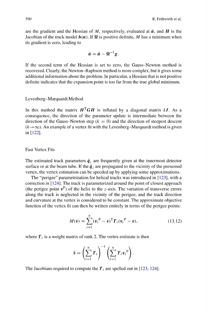
and curvature at the vertex is considered to be constant. The approximate objective
function of the vertex fit can then be written entirely in terms of the perigee points:
M(v) =
n
i=1
(v i
P
− v)
T T i (v i
P
− v),
(13.12)
where T i is a weight matrix of rank 2. The vertex estimate is then
˜
v =
n
i=1
T i
−1 n
i=1
T i v i
P
.
The Jacobians required to compute the T i are spelled out in [123, 124].
R. Frühwirth et al.
are the gradient and the Hessian of M, respectively, evaluated at ˘
α, and H is the
Jacobian of the track model h(α). If is positive definite, M has a minimum when
its gradient is zero, leading to
˜
α = ˘
α −
−1 g.
If the second term of the Hessian is set to zero, the Gauss–Newton method is
recovered. Clearly, the Newton–Raphson method is more complex, but it gives some
additional information about the problem. In particular, a Hessian that is not positive
definite indicates that the expansion point is too far from the true global minimum.
Levenberg–Marquardt Method
In this method the matrix H T GH is inflated by a diagonal matrix kI . As a
consequence, the direction of the parameter update is intermediate between the
direction of the Gauss–Newton step (k = 0) and the direction of steepest descent
(k→∞). An example of a vertex fit with the Levenberg–Marquardt method is given
in [122].
Fast Vertex Fits
The estimated track parameters ˜
q i are frequently given at the innermost detector
surface or at the beam tube. If the ˜
q i are propagated to the vicinity of the presumed
vertex, the vertex estimation can be speeded up by applying some approximations.
The “perigee” parametrization for helical tracks was introduced in [123], with a
correction in [124]. The track is parameterized around the point of closest approach
(the perigee point v P ) of the helix to the z-axis. The variation of transverse errors
along the track is neglected in the vicinity of the perigee, and the track direction
and curvature at the vertex is considered to be constant. The approximate objective
function of the vertex fit can then be written entirely in terms of the perigee points:
M(v) =
n
i=1
(v i
P
− v)
T T i (v i
P
− v),
(13.12)
where T i is a weight matrix of rank 2. The vertex estimate is then
˜
v =
n
i=1
T i
−1 n
i=1
T i v i
P
.
The Jacobians required to compute the T i are spelled out in [123, 124].