

582
R. Frühwirth et al.
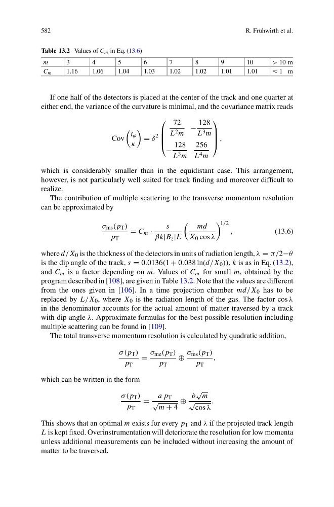
Table 13.2 Values of C m in Eq. (13.6)
m
3
4
5
6
7
8
9
10
> 10 m
C m
1.16
1.06
1.04
1.03
1.02
1.02
1.01
1.01
≈ 1 m
If one half of the detectors is placed at the center of the track and one quarter at
either end, the variance of the curvature is minimal, and the covariance matrix reads
Cov
t ϕ
κ
= δ
2
⎛
⎜
⎜
⎝
72
L 2 m
−
128
L 3 m
−
128
L 3 m
256
L 4 m
⎞
⎟
⎟
⎠ ,
which is considerably smaller than in the equidistant case. This arrangement,
however, is not particularly well suited for track finding and moreover difficult to
realize.
The contribution of multiple scattering to the transverse momentum resolution
can be approximated by
σ ms (p T )
p T
= C m ·
s
βk|B z |L
md
X 0 cos λ
1/2
,
(13.6)
where d/X 0 is the thickness of the detectors in units of radiation length, λ = π/2−θ
is the dip angle of the track, s = 0.0136(1 + 0.038 ln(d/X 0 )), k is as in Eq. (13.2),
and C m is a factor depending on m. Values of C m for small m, obtained by the
program described in [108], are given in Table 13.2. Note that the values are different
from the ones given in [106]. In a time projection chamber md/X 0 has to be
replaced by L/X 0 , where X 0 is the radiation length of the gas. The factor cos λ
in the denominator accounts for the actual amount of matter traversed by a track
with dip angle λ. Approximate formulas for the best possible resolution including
multiple scattering can be found in [109].
The total transverse momentum resolution is calculated by quadratic addition,
σ (p T )
p T
=
σ me (p T )
p T
⊕
σ ms (p T )
p T
,
which can be written in the form
σ (p T )
p T
=
a p T
√
m + 4
⊕
b
√
m
√
cos λ
.
This shows that an optimal m exists for every p T and λ if the projected track length
L is kept fixed. Overinstrumentation will deteriorate the resolution for low momenta
unless additional measurements can be included without increasing the amount of
matter to be traversed.
R. Frühwirth et al.
Table 13.2 Values of C m in Eq. (13.6)
m
3
4
5
6
7
8
9
10
> 10 m
C m
1.16
1.06
1.04
1.03
1.02
1.02
1.01
1.01
≈ 1 m
If one half of the detectors is placed at the center of the track and one quarter at
either end, the variance of the curvature is minimal, and the covariance matrix reads
Cov
t ϕ
κ
= δ
2
⎛
⎜
⎜
⎝
72
L 2 m
−
128
L 3 m
−
128
L 3 m
256
L 4 m
⎞
⎟
⎟
⎠ ,
which is considerably smaller than in the equidistant case. This arrangement,
however, is not particularly well suited for track finding and moreover difficult to
realize.
The contribution of multiple scattering to the transverse momentum resolution
can be approximated by
σ ms (p T )
p T
= C m ·
s
βk|B z |L
md
X 0 cos λ
1/2
,
(13.6)
where d/X 0 is the thickness of the detectors in units of radiation length, λ = π/2−θ
is the dip angle of the track, s = 0.0136(1 + 0.038 ln(d/X 0 )), k is as in Eq. (13.2),
and C m is a factor depending on m. Values of C m for small m, obtained by the
program described in [108], are given in Table 13.2. Note that the values are different
from the ones given in [106]. In a time projection chamber md/X 0 has to be
replaced by L/X 0 , where X 0 is the radiation length of the gas. The factor cos λ
in the denominator accounts for the actual amount of matter traversed by a track
with dip angle λ. Approximate formulas for the best possible resolution including
multiple scattering can be found in [109].
The total transverse momentum resolution is calculated by quadratic addition,
σ (p T )
p T
=
σ me (p T )
p T
⊕
σ ms (p T )
p T
,
which can be written in the form
σ (p T )
p T
=
a p T
√
m + 4
⊕
b
√
m
√
cos λ
.
This shows that an optimal m exists for every p T and λ if the projected track length
L is kept fixed. Overinstrumentation will deteriorate the resolution for low momenta
unless additional measurements can be included without increasing the amount of
matter to be traversed.