

13 Pattern Recognition and Reconstruction
581
where d/X 0 is the thickness of the detectors in units of radiation length. The total
resolution is obtained by adding the corresponding variances and taking the square
root,
σ (p)
p
=
σ me (p)
p
⊕
σ ms (p)
p
= ap ⊕ b,
with a and b depending on the detector and the magnetic field.
13.1.5.2 Cylindrical Spectrometer
Assume that there are m cylindrical detectors immersed in a homogeneous magnetic
field B z parallel to the z axis. The projection of the track on the x–y plane is a circle
with curvature κ. For high momentum the circle can be approximated by a parabola,
the detector cylinders can be approximated by planes, and multiple scattering can
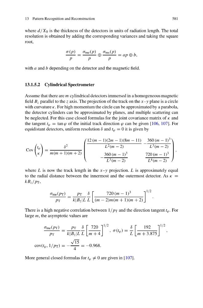
be neglected. For this case closed formulas for the joint covariance matrix of κ and
the tangent t ϕ = tan ϕ of the initial track direction ϕ can be given [106, 107]. For
equidistant detectors, uniform resolution δ and t ϕ = 0 it is given by
Cov
t ϕ
κ
=
δ 2
m(m + 1)(m + 2)
⎛
⎜
⎜
⎜
⎝
12 (m − 1)(2m − 1)(8m − 11)
L 2 (m − 2)
−
360 (m − 1) 3
L 3 (m − 2)
−
360 (m − 1) 3
L 3 (m − 2)
720 (m − 1) 3
L 4 (m − 2)
⎞
⎟
⎟
⎟
⎠
,
where L is now the track length in the x–y projection. L is approximately equal
to the radial distance between the innermost and the outermost detector. As κ =
kB z /p T ,
σ me (p T )
p T
=
p T
k|B z |L
δ
L
720 (m − 1) 3
(m − 2)m(m + 1)(m + 2)
1/2
.
There is a high negative correlation between 1/p T and the direction tangent t ϕ . For
large m, the asymptotic values are
σ me (p T )
p T
=
p T
k|B z |L
δ
L
720
m + 4
1/2
, σ(t ϕ ) =
δ
L
192
m + 3.875
1/2
,
cov(t ϕ , 1/p T ) = −
√
15
4
= −0.968.
More general closed formulas for t ϕ = 0 are given in [107].
581
where d/X 0 is the thickness of the detectors in units of radiation length. The total
resolution is obtained by adding the corresponding variances and taking the square
root,
σ (p)
p
=
σ me (p)
p
⊕
σ ms (p)
p
= ap ⊕ b,
with a and b depending on the detector and the magnetic field.
13.1.5.2 Cylindrical Spectrometer
Assume that there are m cylindrical detectors immersed in a homogeneous magnetic
field B z parallel to the z axis. The projection of the track on the x–y plane is a circle
with curvature κ. For high momentum the circle can be approximated by a parabola,
the detector cylinders can be approximated by planes, and multiple scattering can
be neglected. For this case closed formulas for the joint covariance matrix of κ and
the tangent t ϕ = tan ϕ of the initial track direction ϕ can be given [106, 107]. For
equidistant detectors, uniform resolution δ and t ϕ = 0 it is given by
Cov
t ϕ
κ
=
δ 2
m(m + 1)(m + 2)
⎛
⎜
⎜
⎜
⎝
12 (m − 1)(2m − 1)(8m − 11)
L 2 (m − 2)
−
360 (m − 1) 3
L 3 (m − 2)
−
360 (m − 1) 3
L 3 (m − 2)
720 (m − 1) 3
L 4 (m − 2)
⎞
⎟
⎟
⎟
⎠
,
where L is now the track length in the x–y projection. L is approximately equal
to the radial distance between the innermost and the outermost detector. As κ =
kB z /p T ,
σ me (p T )
p T
=
p T
k|B z |L
δ
L
720 (m − 1) 3
(m − 2)m(m + 1)(m + 2)
1/2
.
There is a high negative correlation between 1/p T and the direction tangent t ϕ . For
large m, the asymptotic values are
σ me (p T )
p T
=
p T
k|B z |L
δ
L
720
m + 4
1/2
, σ(t ϕ ) =
δ
L
192
m + 3.875
1/2
,
cov(t ϕ , 1/p T ) = −
√
15
4
= −0.968.
More general closed formulas for t ϕ = 0 are given in [107].