

13 Pattern Recognition and Reconstruction
571
small matrices and exhibits the same attractive feature as the breakpoint method of
following the actual track quite closely [26, 60].
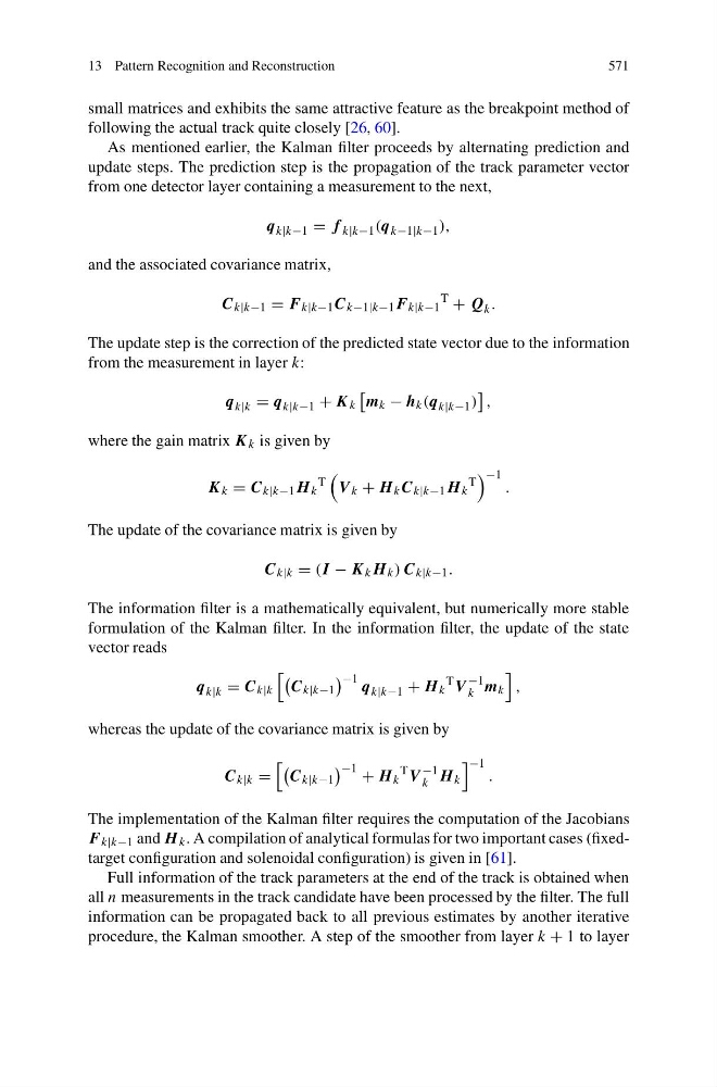
As mentioned earlier, the Kalman filter proceeds by alternating prediction and
update steps. The prediction step is the propagation of the track parameter vector
from one detector layer containing a measurement to the next,
q k|k−1 = f k|k−1 (q k−1|k−1 ),
and the associated covariance matrix,
C k|k−1 = F k|k−1 C k−1|k−1 F k|k−1
T
+ Q k .
The update step is the correction of the predicted state vector due to the information
from the measurement in layer k:
q k|k = q k|k−1 + K k
m k − h k (q k|k−1 )
,
where the gain matrix K k is given by
K k = C k|k−1 H k
T
V k + H k C k|k−1 H k
T
−1
.
The update of the covariance matrix is given by
C k|k = (I − K k H k ) C k|k−1 .
The information filter is a mathematically equivalent, but numerically more stable
formulation of the Kalman filter. In the information filter, the update of the state
vector reads
q k|k = C k|k
C k|k−1
−1 q k|k−1 + H k
T V
−1
k m k
,
whereas the update of the covariance matrix is given by
C k|k =
C k|k−1
−1 + H k
T V
−1
k H k
−1
.
The implementation of the Kalman filter requires the computation of the Jacobians
F k|k−1 and H k . A compilation of analytical formulas for two important cases (fixedtarget configuration and solenoidal configuration) is given in [61].
Full information of the track parameters at the end of the track is obtained when
all n measurements in the track candidate have been processed by the filter. The full
information can be propagated back to all previous estimates by another iterative
procedure, the Kalman smoother. A step of the smoother from layer k + 1 to layer
571
small matrices and exhibits the same attractive feature as the breakpoint method of
following the actual track quite closely [26, 60].
As mentioned earlier, the Kalman filter proceeds by alternating prediction and
update steps. The prediction step is the propagation of the track parameter vector
from one detector layer containing a measurement to the next,
q k|k−1 = f k|k−1 (q k−1|k−1 ),
and the associated covariance matrix,
C k|k−1 = F k|k−1 C k−1|k−1 F k|k−1
T
+ Q k .
The update step is the correction of the predicted state vector due to the information
from the measurement in layer k:
q k|k = q k|k−1 + K k
m k − h k (q k|k−1 )
,
where the gain matrix K k is given by
K k = C k|k−1 H k
T
V k + H k C k|k−1 H k
T
−1
.
The update of the covariance matrix is given by
C k|k = (I − K k H k ) C k|k−1 .
The information filter is a mathematically equivalent, but numerically more stable
formulation of the Kalman filter. In the information filter, the update of the state
vector reads
q k|k = C k|k
C k|k−1
−1 q k|k−1 + H k
T V
−1
k m k
,
whereas the update of the covariance matrix is given by
C k|k =
C k|k−1
−1 + H k
T V
−1
k H k
−1
.
The implementation of the Kalman filter requires the computation of the Jacobians
F k|k−1 and H k . A compilation of analytical formulas for two important cases (fixedtarget configuration and solenoidal configuration) is given in [61].
Full information of the track parameters at the end of the track is obtained when
all n measurements in the track candidate have been processed by the filter. The full
information can be propagated back to all previous estimates by another iterative
procedure, the Kalman smoother. A step of the smoother from layer k + 1 to layer