

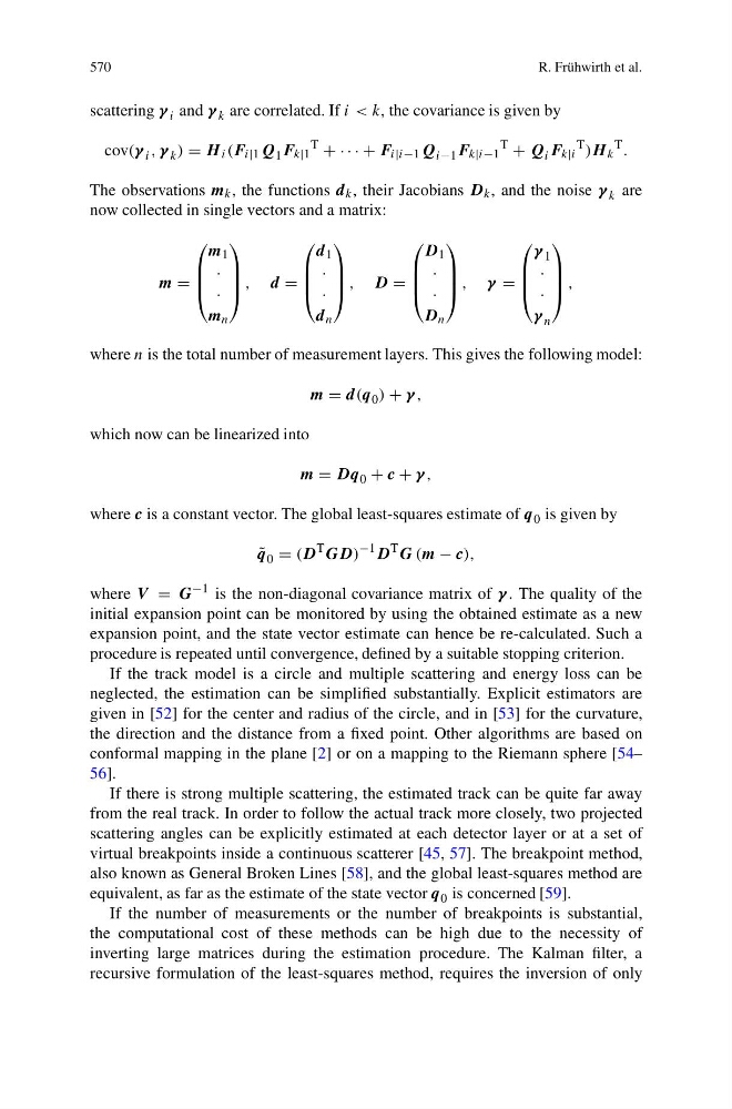
570
R. Frühwirth et al.
scattering γ i and γ k are correlated. If i < k, the covariance is given by
cov(γ i , γ k ) = H i (F i|1 Q 1 F k|1
T
+ · · · + F i|i−1 Q i−1 F k|i−1
T
+ Q i F k|i
T )H k
T .
The observations m k , the functions d k , their Jacobians D k , and the noise γ k are
now collected in single vectors and a matrix:
m =
⎛
⎜
⎜
⎝
m 1
·
·
m n
⎞
⎟
⎟
⎠ , d =
⎛
⎜
⎜
⎝
d 1
·
·
d n
⎞
⎟
⎟
⎠ , D =
⎛
⎜
⎜
⎝
D 1
·
·
D n
⎞
⎟
⎟
⎠ , γ =
⎛
⎜
⎜
⎝
γ 1
·
·
γ n
⎞
⎟
⎟
⎠ ,
where n is the total number of measurement layers. This gives the following model:
m = d(q 0 ) + γ ,
which now can be linearized into
m = Dq 0 + c + γ ,
where c is a constant vector. The global least-squares estimate of q 0 is given by
˜
q 0 = (D
T GD)
−1 D
T G (m − c),
where V = G
−1 is the non-diagonal covariance matrix of γ . The quality of the
initial expansion point can be monitored by using the obtained estimate as a new
expansion point, and the state vector estimate can hence be re-calculated. Such a
procedure is repeated until convergence, defined by a suitable stopping criterion.
If the track model is a circle and multiple scattering and energy loss can be
neglected, the estimation can be simplified substantially. Explicit estimators are
given in [52] for the center and radius of the circle, and in [53] for the curvature,
the direction and the distance from a fixed point. Other algorithms are based on
conformal mapping in the plane [2] or on a mapping to the Riemann sphere [54–
56].
If there is strong multiple scattering, the estimated track can be quite far away
from the real track. In order to follow the actual track more closely, two projected
scattering angles can be explicitly estimated at each detector layer or at a set of
virtual breakpoints inside a continuous scatterer [45, 57]. The breakpoint method,
also known as General Broken Lines [58], and the global least-squares method are
equivalent, as far as the estimate of the state vector q 0 is concerned [59].
If the number of measurements or the number of breakpoints is substantial,
the computational cost of these methods can be high due to the necessity of
inverting large matrices during the estimation procedure. The Kalman filter, a
recursive formulation of the least-squares method, requires the inversion of only
R. Frühwirth et al.
scattering γ i and γ k are correlated. If i < k, the covariance is given by
cov(γ i , γ k ) = H i (F i|1 Q 1 F k|1
T
+ · · · + F i|i−1 Q i−1 F k|i−1
T
+ Q i F k|i
T )H k
T .
The observations m k , the functions d k , their Jacobians D k , and the noise γ k are
now collected in single vectors and a matrix:
m =
⎛
⎜
⎜
⎝
m 1
·
·
m n
⎞
⎟
⎟
⎠ , d =
⎛
⎜
⎜
⎝
d 1
·
·
d n
⎞
⎟
⎟
⎠ , D =
⎛
⎜
⎜
⎝
D 1
·
·
D n
⎞
⎟
⎟
⎠ , γ =
⎛
⎜
⎜
⎝
γ 1
·
·
γ n
⎞
⎟
⎟
⎠ ,
where n is the total number of measurement layers. This gives the following model:
m = d(q 0 ) + γ ,
which now can be linearized into
m = Dq 0 + c + γ ,
where c is a constant vector. The global least-squares estimate of q 0 is given by
˜
q 0 = (D
T GD)
−1 D
T G (m − c),
where V = G
−1 is the non-diagonal covariance matrix of γ . The quality of the
initial expansion point can be monitored by using the obtained estimate as a new
expansion point, and the state vector estimate can hence be re-calculated. Such a
procedure is repeated until convergence, defined by a suitable stopping criterion.
If the track model is a circle and multiple scattering and energy loss can be
neglected, the estimation can be simplified substantially. Explicit estimators are
given in [52] for the center and radius of the circle, and in [53] for the curvature,
the direction and the distance from a fixed point. Other algorithms are based on
conformal mapping in the plane [2] or on a mapping to the Riemann sphere [54–
56].
If there is strong multiple scattering, the estimated track can be quite far away
from the real track. In order to follow the actual track more closely, two projected
scattering angles can be explicitly estimated at each detector layer or at a set of
virtual breakpoints inside a continuous scatterer [45, 57]. The breakpoint method,
also known as General Broken Lines [58], and the global least-squares method are
equivalent, as far as the estimate of the state vector q 0 is concerned [59].
If the number of measurements or the number of breakpoints is substantial,
the computational cost of these methods can be high due to the necessity of
inverting large matrices during the estimation procedure. The Kalman filter, a
recursive formulation of the least-squares method, requires the inversion of only