

562
R. Frühwirth et al.
equations. Field measurements inside the volume are used to evaluate the quality
of the calculated field. If the measurements inside the volume are precise enough,
they can be used to further refine the knowledge of the field by being included in
the estimation procedure of the abovementioned coefficients [34].
In a track reconstruction application, fast access to the value of the magnetic
field at any point inside the detector volume is crucial. For this purpose, a numerical
representation of the field is needed. A frequently used approach is to create a table
of the magnetic field values at a grid of points and to determine the field at points
between the grid nodes by linear or quadratic interpolation. An alternative approach
is to divide the detector volume into several sub-volumes and to fit the coefficients
of low-order polynomials to the known field values inside each sub-volume [35,
36]. If the number of sub-volumes is large, potentially many coefficients have to
be determined. On the other hand, once the coefficients are determined, the field
access is very fast. Also, the derivatives of the field, which are needed by some
track reconstruction algorithms, can be computed as fast as the field itself.
13.1.3.2 Track Models
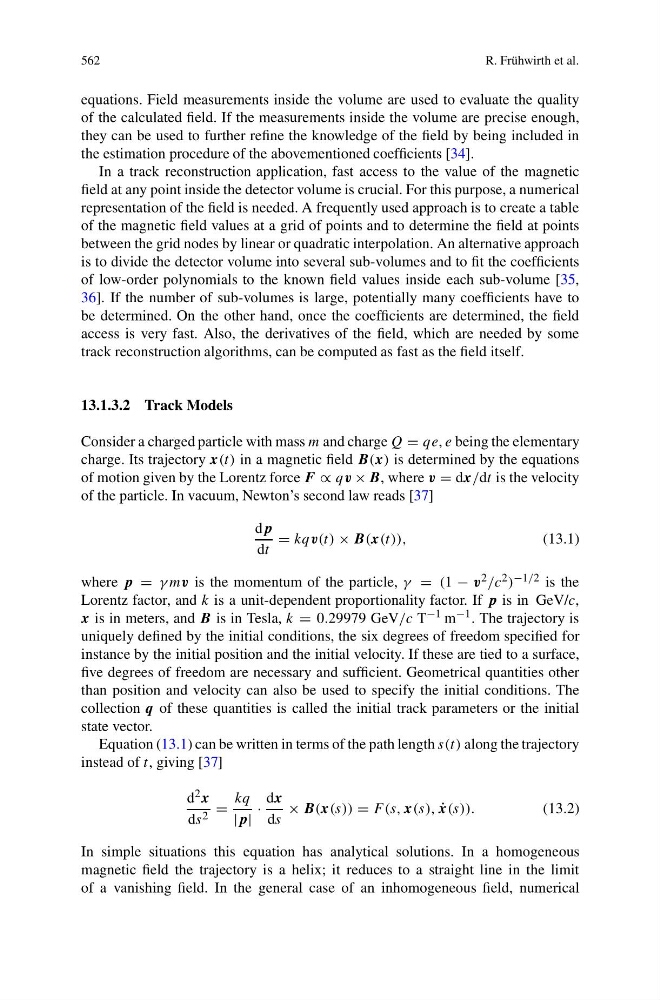
Consider a charged particle with mass m and charge Q = qe, e being the elementary
charge. Its trajectory x(t) in a magnetic field B(x) is determined by the equations
of motion given by the Lorentz force F ∝ qv × B, where v = dx/dt is the velocity
of the particle. In vacuum, Newton’s second law reads [37]
dp
dt
= kqv(t) × B(x(t)),
(13.1)
where p = γ mv is the momentum of the particle, γ = (1 − v 2 /c 2 ) −1/2 is the
Lorentz factor, and k is a unit-dependent proportionality factor. If p is in GeV/c,
x is in meters, and B is in Tesla, k = 0.29979 GeV/c T −1 m −1 . The trajectory is
uniquely defined by the initial conditions, the six degrees of freedom specified for
instance by the initial position and the initial velocity. If these are tied to a surface,
five degrees of freedom are necessary and sufficient. Geometrical quantities other
than position and velocity can also be used to specify the initial conditions. The
collection q of these quantities is called the initial track parameters or the initial
state vector.
Equation (13.1) can be written in terms of the path length s(t) along the trajectory
instead of t, giving [37]
d 2 x
ds 2 =
kq
|p|
·
dx
ds
× B(x(s)) = F (s, x(s), ˙
x(s)).
(13.2)
In simple situations this equation has analytical solutions. In a homogeneous
magnetic field the trajectory is a helix; it reduces to a straight line in the limit
of a vanishing field. In the general case of an inhomogeneous field, numerical
R. Frühwirth et al.
equations. Field measurements inside the volume are used to evaluate the quality
of the calculated field. If the measurements inside the volume are precise enough,
they can be used to further refine the knowledge of the field by being included in
the estimation procedure of the abovementioned coefficients [34].
In a track reconstruction application, fast access to the value of the magnetic
field at any point inside the detector volume is crucial. For this purpose, a numerical
representation of the field is needed. A frequently used approach is to create a table
of the magnetic field values at a grid of points and to determine the field at points
between the grid nodes by linear or quadratic interpolation. An alternative approach
is to divide the detector volume into several sub-volumes and to fit the coefficients
of low-order polynomials to the known field values inside each sub-volume [35,
36]. If the number of sub-volumes is large, potentially many coefficients have to
be determined. On the other hand, once the coefficients are determined, the field
access is very fast. Also, the derivatives of the field, which are needed by some
track reconstruction algorithms, can be computed as fast as the field itself.
13.1.3.2 Track Models
Consider a charged particle with mass m and charge Q = qe, e being the elementary
charge. Its trajectory x(t) in a magnetic field B(x) is determined by the equations
of motion given by the Lorentz force F ∝ qv × B, where v = dx/dt is the velocity
of the particle. In vacuum, Newton’s second law reads [37]
dp
dt
= kqv(t) × B(x(t)),
(13.1)
where p = γ mv is the momentum of the particle, γ = (1 − v 2 /c 2 ) −1/2 is the
Lorentz factor, and k is a unit-dependent proportionality factor. If p is in GeV/c,
x is in meters, and B is in Tesla, k = 0.29979 GeV/c T −1 m −1 . The trajectory is
uniquely defined by the initial conditions, the six degrees of freedom specified for
instance by the initial position and the initial velocity. If these are tied to a surface,
five degrees of freedom are necessary and sufficient. Geometrical quantities other
than position and velocity can also be used to specify the initial conditions. The
collection q of these quantities is called the initial track parameters or the initial
state vector.
Equation (13.1) can be written in terms of the path length s(t) along the trajectory
instead of t, giving [37]
d 2 x
ds 2 =
kq
|p|
·
dx
ds
× B(x(s)) = F (s, x(s), ˙
x(s)).
(13.2)
In simple situations this equation has analytical solutions. In a homogeneous
magnetic field the trajectory is a helix; it reduces to a straight line in the limit
of a vanishing field. In the general case of an inhomogeneous field, numerical