

13 Pattern Recognition and Reconstruction
563
methods can be used, such as Runge–Kutta integration of the equations of motion or
parametrization by polynomials or splines [37]. Among Runge–Kutta methods, the
Runge-Kutta-Nyström algorithm is specially designed for second-order equations
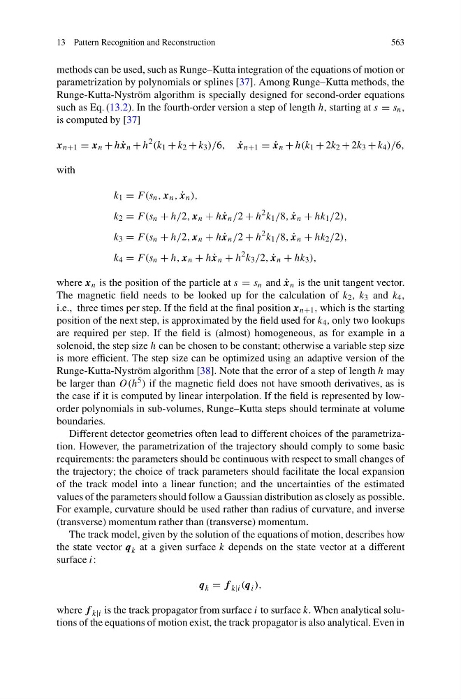
such as Eq. (13.2). In the fourth-order version a step of length h, starting at s = s n ,
is computed by [37]
x n+1 = x n + h ˙
x n + h
2 (k 1 + k 2 + k 3 )/6, ˙
x n+1 = ˙
x n + h(k 1 + 2k 2 + 2k 3 + k 4 )/6,
with
k 1 = F (s n , x n , ˙
x n ),
k 2 = F (s n + h/2, x n + h ˙
x n /2 + h
2 k 1 /8, ˙
x n + hk 1 /2),
k 3 = F (s n + h/2, x n + h ˙
x n /2 + h
2 k 1 /8, ˙
x n + hk 2 /2),
k 4 = F (s n + h, x n + h ˙
x n + h
2 k 3 /2, ˙
x n + hk 3 ),
where x n is the position of the particle at s = s n and ˙
x n is the unit tangent vector.
The magnetic field needs to be looked up for the calculation of k 2 , k 3 and k 4 ,
i.e., three times per step. If the field at the final position x n+1 , which is the starting
position of the next step, is approximated by the field used for k 4 , only two lookups
are required per step. If the field is (almost) homogeneous, as for example in a
solenoid, the step size h can be chosen to be constant; otherwise a variable step size
is more efficient. The step size can be optimized using an adaptive version of the
Runge-Kutta-Nyström algorithm [38]. Note that the error of a step of length h may
be larger than O(h 5 ) if the magnetic field does not have smooth derivatives, as is
the case if it is computed by linear interpolation. If the field is represented by loworder polynomials in sub-volumes, Runge–Kutta steps should terminate at volume
boundaries.
Different detector geometries often lead to different choices of the parametrization. However, the parametrization of the trajectory should comply to some basic
requirements: the parameters should be continuous with respect to small changes of
the trajectory; the choice of track parameters should facilitate the local expansion
of the track model into a linear function; and the uncertainties of the estimated
values of the parameters should follow a Gaussian distribution as closely as possible.
For example, curvature should be used rather than radius of curvature, and inverse
(transverse) momentum rather than (transverse) momentum.
The track model, given by the solution of the equations of motion, describes how
the state vector q k at a given surface k depends on the state vector at a different
surface i:
q k = f k|i (q i ),
where f k|i is the track propagator from surface i to surface k. When analytical solutions of the equations of motion exist, the track propagator is also analytical. Even in
563
methods can be used, such as Runge–Kutta integration of the equations of motion or
parametrization by polynomials or splines [37]. Among Runge–Kutta methods, the
Runge-Kutta-Nyström algorithm is specially designed for second-order equations
such as Eq. (13.2). In the fourth-order version a step of length h, starting at s = s n ,
is computed by [37]
x n+1 = x n + h ˙
x n + h
2 (k 1 + k 2 + k 3 )/6, ˙
x n+1 = ˙
x n + h(k 1 + 2k 2 + 2k 3 + k 4 )/6,
with
k 1 = F (s n , x n , ˙
x n ),
k 2 = F (s n + h/2, x n + h ˙
x n /2 + h
2 k 1 /8, ˙
x n + hk 1 /2),
k 3 = F (s n + h/2, x n + h ˙
x n /2 + h
2 k 1 /8, ˙
x n + hk 2 /2),
k 4 = F (s n + h, x n + h ˙
x n + h
2 k 3 /2, ˙
x n + hk 3 ),
where x n is the position of the particle at s = s n and ˙
x n is the unit tangent vector.
The magnetic field needs to be looked up for the calculation of k 2 , k 3 and k 4 ,
i.e., three times per step. If the field at the final position x n+1 , which is the starting
position of the next step, is approximated by the field used for k 4 , only two lookups
are required per step. If the field is (almost) homogeneous, as for example in a
solenoid, the step size h can be chosen to be constant; otherwise a variable step size
is more efficient. The step size can be optimized using an adaptive version of the
Runge-Kutta-Nyström algorithm [38]. Note that the error of a step of length h may
be larger than O(h 5 ) if the magnetic field does not have smooth derivatives, as is
the case if it is computed by linear interpolation. If the field is represented by loworder polynomials in sub-volumes, Runge–Kutta steps should terminate at volume
boundaries.
Different detector geometries often lead to different choices of the parametrization. However, the parametrization of the trajectory should comply to some basic
requirements: the parameters should be continuous with respect to small changes of
the trajectory; the choice of track parameters should facilitate the local expansion
of the track model into a linear function; and the uncertainties of the estimated
values of the parameters should follow a Gaussian distribution as closely as possible.
For example, curvature should be used rather than radius of curvature, and inverse
(transverse) momentum rather than (transverse) momentum.
The track model, given by the solution of the equations of motion, describes how
the state vector q k at a given surface k depends on the state vector at a different
surface i:
q k = f k|i (q i ),
where f k|i is the track propagator from surface i to surface k. When analytical solutions of the equations of motion exist, the track propagator is also analytical. Even in