

13 Pattern Recognition and Reconstruction
561
from seed
Reject
Accept
A
B
C
D
E
T2
T1
T3
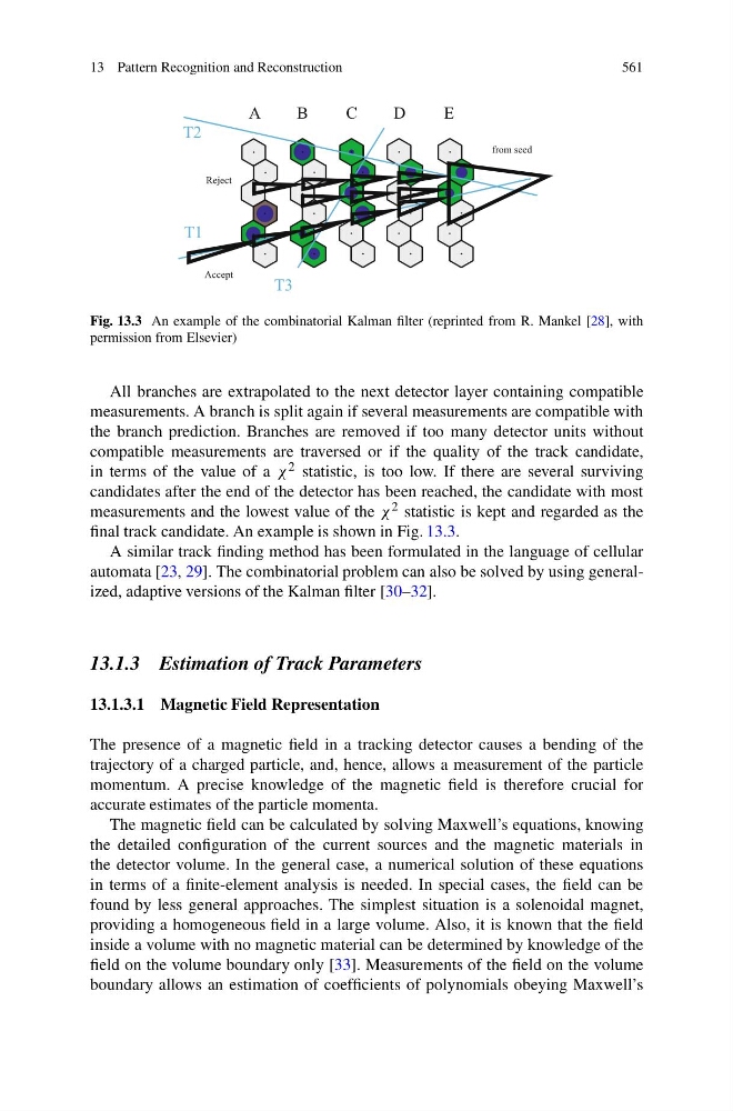
Fig. 13.3 An example of the combinatorial Kalman filter (reprinted from R. Mankel [28], with
permission from Elsevier)
All branches are extrapolated to the next detector layer containing compatible
measurements. A branch is split again if several measurements are compatible with
the branch prediction. Branches are removed if too many detector units without
compatible measurements are traversed or if the quality of the track candidate,
in terms of the value of a χ 2 statistic, is too low. If there are several surviving
candidates after the end of the detector has been reached, the candidate with most
measurements and the lowest value of the χ 2 statistic is kept and regarded as the
final track candidate. An example is shown in Fig. 13.3.
A similar track finding method has been formulated in the language of cellular
automata [23, 29]. The combinatorial problem can also be solved by using generalized, adaptive versions of the Kalman filter [30–32].
13.1.3 Estimation of Track Parameters
13.1.3.1 Magnetic Field Representation
The presence of a magnetic field in a tracking detector causes a bending of the
trajectory of a charged particle, and, hence, allows a measurement of the particle
momentum. A precise knowledge of the magnetic field is therefore crucial for
accurate estimates of the particle momenta.
The magnetic field can be calculated by solving Maxwell’s equations, knowing
the detailed configuration of the current sources and the magnetic materials in
the detector volume. In the general case, a numerical solution of these equations
in terms of a finite-element analysis is needed. In special cases, the field can be
found by less general approaches. The simplest situation is a solenoidal magnet,
providing a homogeneous field in a large volume. Also, it is known that the field
inside a volume with no magnetic material can be determined by knowledge of the
field on the volume boundary only [33]. Measurements of the field on the volume
boundary allows an estimation of coefficients of polynomials obeying Maxwell’s
561
from seed
Reject
Accept
A
B
C
D
E
T2
T1
T3
Fig. 13.3 An example of the combinatorial Kalman filter (reprinted from R. Mankel [28], with
permission from Elsevier)
All branches are extrapolated to the next detector layer containing compatible
measurements. A branch is split again if several measurements are compatible with
the branch prediction. Branches are removed if too many detector units without
compatible measurements are traversed or if the quality of the track candidate,
in terms of the value of a χ 2 statistic, is too low. If there are several surviving
candidates after the end of the detector has been reached, the candidate with most
measurements and the lowest value of the χ 2 statistic is kept and regarded as the
final track candidate. An example is shown in Fig. 13.3.
A similar track finding method has been formulated in the language of cellular
automata [23, 29]. The combinatorial problem can also be solved by using generalized, adaptive versions of the Kalman filter [30–32].
13.1.3 Estimation of Track Parameters
13.1.3.1 Magnetic Field Representation
The presence of a magnetic field in a tracking detector causes a bending of the
trajectory of a charged particle, and, hence, allows a measurement of the particle
momentum. A precise knowledge of the magnetic field is therefore crucial for
accurate estimates of the particle momenta.
The magnetic field can be calculated by solving Maxwell’s equations, knowing
the detailed configuration of the current sources and the magnetic materials in
the detector volume. In the general case, a numerical solution of these equations
in terms of a finite-element analysis is needed. In special cases, the field can be
found by less general approaches. The simplest situation is a solenoidal magnet,
providing a homogeneous field in a large volume. Also, it is known that the field
inside a volume with no magnetic material can be determined by knowledge of the
field on the volume boundary only [33]. Measurements of the field on the volume
boundary allows an estimation of coefficients of polynomials obeying Maxwell’s