

468
V. Radeka
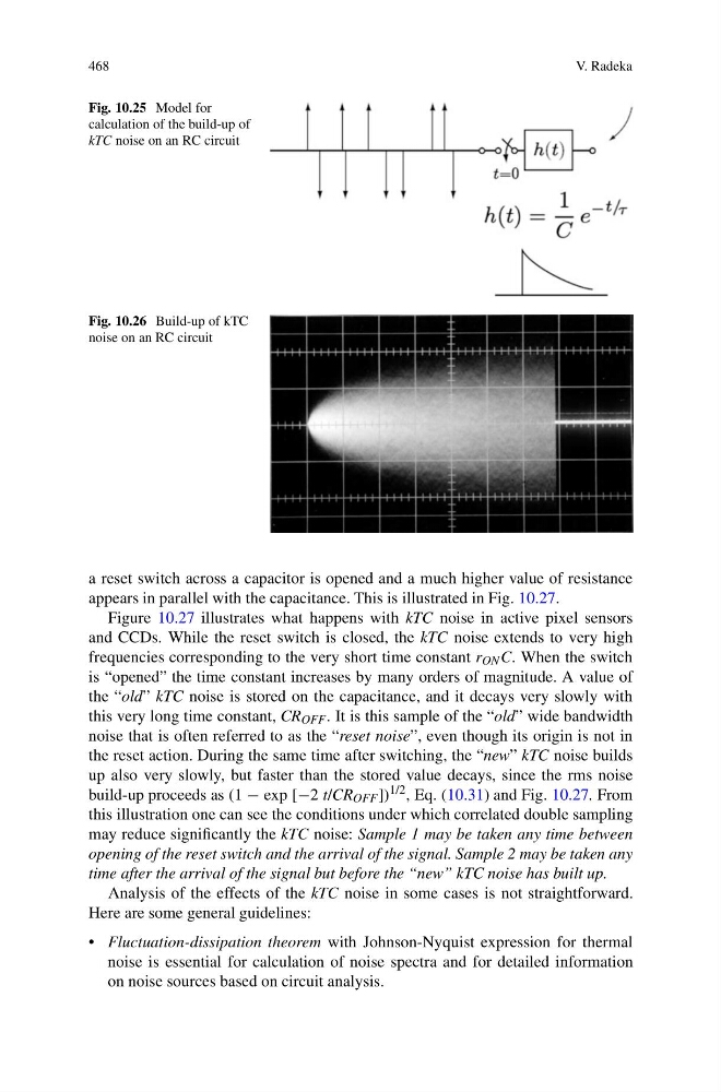
Fig. 10.25 Model for
calculation of the build-up of
kTC noise on an RC circuit
Fig. 10.26 Build-up of kTC
noise on an RC circuit
a reset switch across a capacitor is opened and a much higher value of resistance
appears in parallel with the capacitance. This is illustrated in Fig. 10.27.
Figure 10.27 illustrates what happens with kTC noise in active pixel sensors
and CCDs. While the reset switch is closed, the kTC noise extends to very high
frequencies corresponding to the very short time constant r ON C. When the switch
is “opened” the time constant increases by many orders of magnitude. A value of
the “old” kTC noise is stored on the capacitance, and it decays very slowly with
this very long time constant, CR OFF . It is this sample of the “old” wide bandwidth
noise that is often referred to as the “reset noise”, even though its origin is not in
the reset action. During the same time after switching, the “new” kTC noise builds
up also very slowly, but faster than the stored value decays, since the rms noise
build-up proceeds as (1 − exp [−2 t/CR OFF ]) 1/2 , Eq. (10.31) and Fig. 10.27. From
this illustration one can see the conditions under which correlated double sampling
may reduce significantly the kTC noise: Sample 1 may be taken any time between
opening of the reset switch and the arrival of the signal. Sample 2 may be taken any
time after the arrival of the signal but before the “new” kTC noise has built up.
Analysis of the effects of the kTC noise in some cases is not straightforward.
Here are some general guidelines:
• Fluctuation-dissipation theorem with Johnson-Nyquist expression for thermal
noise is essential for calculation of noise spectra and for detailed information
on noise sources based on circuit analysis.
V. Radeka
Fig. 10.25 Model for
calculation of the build-up of
kTC noise on an RC circuit
Fig. 10.26 Build-up of kTC
noise on an RC circuit
a reset switch across a capacitor is opened and a much higher value of resistance
appears in parallel with the capacitance. This is illustrated in Fig. 10.27.
Figure 10.27 illustrates what happens with kTC noise in active pixel sensors
and CCDs. While the reset switch is closed, the kTC noise extends to very high
frequencies corresponding to the very short time constant r ON C. When the switch
is “opened” the time constant increases by many orders of magnitude. A value of
the “old” kTC noise is stored on the capacitance, and it decays very slowly with
this very long time constant, CR OFF . It is this sample of the “old” wide bandwidth
noise that is often referred to as the “reset noise”, even though its origin is not in
the reset action. During the same time after switching, the “new” kTC noise builds
up also very slowly, but faster than the stored value decays, since the rms noise
build-up proceeds as (1 − exp [−2 t/CR OFF ]) 1/2 , Eq. (10.31) and Fig. 10.27. From
this illustration one can see the conditions under which correlated double sampling
may reduce significantly the kTC noise: Sample 1 may be taken any time between
opening of the reset switch and the arrival of the signal. Sample 2 may be taken any
time after the arrival of the signal but before the “new” kTC noise has built up.
Analysis of the effects of the kTC noise in some cases is not straightforward.
Here are some general guidelines:
• Fluctuation-dissipation theorem with Johnson-Nyquist expression for thermal
noise is essential for calculation of noise spectra and for detailed information
on noise sources based on circuit analysis.