

7 Particle Detectors and Detector Systems
291
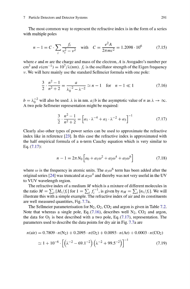
The most common way to represent the refractive index is in the form of a series
with multiple poles
n − 1 = C ·
i
f i
ν 2
i − ν 2
with C =
e 2 A
2πmc 2 = 1.2098 · 10
6
(7.15)
where e and m are the charge and mass of the electron, A is Avogadro’s number per
cm 3 and ν(cm −1 ) = 10 7 /λ(nm). f i is the oscillator strength of the Eigen frequency
ν. We will here mainly use the standard Sellmeier formula with one pole:
3
2
·
n 2 − 1
n 2 + 2
=
a
λ
−2
0 − λ −2
n − 1 for n − 1 1
(7.16)
b = λ
−2
0 will also be used. λ is in nm. a/b is the asymptotic value of n as λ → ∞.
A two pole Sellmeier representation might be required:
3
2
·
n 2 − 1
n 2 + 2
=
a 1 · λ
−4
+ a 2 · λ
−2
+ a 3
−1
(7.17)
Clearly also other types of power series can be used to approximate the refractive
index like in reference [23]. In this case the refractive index is approximated with
the half empirical formula of a n-term Cauchy equation which is very similar to
Eq. (7.17):
n − 1 = 2πN 0
a 0 + a 1 ω
2
+ a 2 ω
4
+ a 3 ω
6
(7.18)
where ω is the frequency in atomic units. The a 3 ω 6 term has been added after the
original series [24] was truncated at a 2 ω 4 and thereby was not very useful in the UV
to VUV wavelength region.
The refractive index of a medium M which is a mixture of different molecules in
the ratio M =
i [M i /f i ] for 1 =
i f
−1
i , is given by n M =
i [n i /f i ]. We will
illustrate this with a simple example. The refractive index of air and its constituents
are well measured quantities, Fig. 7.7a.
The Sellmeier parameterisation for N 2 , O 2 , CO 2 and argon is given in Table 7.2.
Note that whereas a single pole, Eq. (7.16), describes well N 2 , CO 2 and argon,
the data for O 2 is best described with a two pole, Eq. (7.17), representation. The
parameters used to describe the data points for dry air in Fig. 7.7a are
n(air) = 0.7809 · n(N 2 ) + 0.2095 · n(O 2 ) + 0.0093 · n(Ar) + 0.0003 · n(CO 2 )
1 + 10
−6
·
λ
−2
− 69.1
−2
λ
−2
+ 99.5
−2
−1
(7.19)
291
The most common way to represent the refractive index is in the form of a series
with multiple poles
n − 1 = C ·
i
f i
ν 2
i − ν 2
with C =
e 2 A
2πmc 2 = 1.2098 · 10
6
(7.15)
where e and m are the charge and mass of the electron, A is Avogadro’s number per
cm 3 and ν(cm −1 ) = 10 7 /λ(nm). f i is the oscillator strength of the Eigen frequency
ν. We will here mainly use the standard Sellmeier formula with one pole:
3
2
·
n 2 − 1
n 2 + 2
=
a
λ
−2
0 − λ −2
n − 1 for n − 1 1
(7.16)
b = λ
−2
0 will also be used. λ is in nm. a/b is the asymptotic value of n as λ → ∞.
A two pole Sellmeier representation might be required:
3
2
·
n 2 − 1
n 2 + 2
=
a 1 · λ
−4
+ a 2 · λ
−2
+ a 3
−1
(7.17)
Clearly also other types of power series can be used to approximate the refractive
index like in reference [23]. In this case the refractive index is approximated with
the half empirical formula of a n-term Cauchy equation which is very similar to
Eq. (7.17):
n − 1 = 2πN 0
a 0 + a 1 ω
2
+ a 2 ω
4
+ a 3 ω
6
(7.18)
where ω is the frequency in atomic units. The a 3 ω 6 term has been added after the
original series [24] was truncated at a 2 ω 4 and thereby was not very useful in the UV
to VUV wavelength region.
The refractive index of a medium M which is a mixture of different molecules in
the ratio M =
i [M i /f i ] for 1 =
i f
−1
i , is given by n M =
i [n i /f i ]. We will
illustrate this with a simple example. The refractive index of air and its constituents
are well measured quantities, Fig. 7.7a.
The Sellmeier parameterisation for N 2 , O 2 , CO 2 and argon is given in Table 7.2.
Note that whereas a single pole, Eq. (7.16), describes well N 2 , CO 2 and argon,
the data for O 2 is best described with a two pole, Eq. (7.17), representation. The
parameters used to describe the data points for dry air in Fig. 7.7a are
n(air) = 0.7809 · n(N 2 ) + 0.2095 · n(O 2 ) + 0.0093 · n(Ar) + 0.0003 · n(CO 2 )
1 + 10
−6
·
λ
−2
− 69.1
−2
λ
−2
+ 99.5
−2
−1
(7.19)