

80
W. Herr and E. Forest
: H :
3 x = 2k(xp x − yp y ),
(3.102)
. . . .
(3.103)
Putting the terms together one obtains:
e −L : H : x = x + p x L −
1
2
kL
2 (x
2
− y
2 ) −
1
3
kL
3 (xp x − yp y ) + . . .
(3.104)
3.7.4 Analysis Techniques: Poincare Surface of Section
Under normal circumstances it is not required to examine the complete time
development of a particle trajectory around the machine. Given the experimental
fact that the trajectory can be measured only at a finite number of positions around
the machine, it is only useful to sample the trajectory periodically at a fixed position.
The plot of the rate of change of the phase space variables at the beginning (or
end) of each period is the appropriate method and also known as Poincare Surface
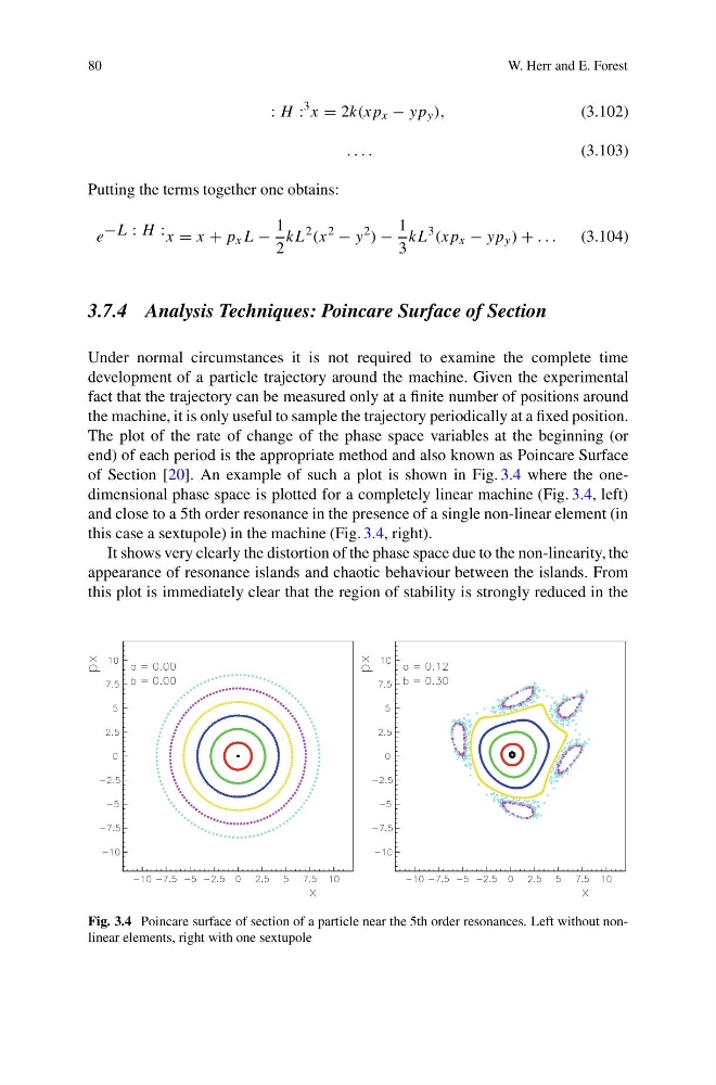
of Section [20]. An example of such a plot is shown in Fig. 3.4 where the onedimensional phase space is plotted for a completely linear machine (Fig. 3.4, left)
and close to a 5th order resonance in the presence of a single non-linear element (in
this case a sextupole) in the machine (Fig. 3.4, right).
It shows very clearly the distortion of the phase space due to the non-linearity, the
appearance of resonance islands and chaotic behaviour between the islands. From
this plot is immediately clear that the region of stability is strongly reduced in the
Fig. 3.4 Poincare surface of section of a particle near the 5th order resonances. Left without nonlinear elements, right with one sextupole
W. Herr and E. Forest
: H :
3 x = 2k(xp x − yp y ),
(3.102)
. . . .
(3.103)
Putting the terms together one obtains:
e −L : H : x = x + p x L −
1
2
kL
2 (x
2
− y
2 ) −
1
3
kL
3 (xp x − yp y ) + . . .
(3.104)
3.7.4 Analysis Techniques: Poincare Surface of Section
Under normal circumstances it is not required to examine the complete time
development of a particle trajectory around the machine. Given the experimental
fact that the trajectory can be measured only at a finite number of positions around
the machine, it is only useful to sample the trajectory periodically at a fixed position.
The plot of the rate of change of the phase space variables at the beginning (or
end) of each period is the appropriate method and also known as Poincare Surface
of Section [20]. An example of such a plot is shown in Fig. 3.4 where the onedimensional phase space is plotted for a completely linear machine (Fig. 3.4, left)
and close to a 5th order resonance in the presence of a single non-linear element (in
this case a sextupole) in the machine (Fig. 3.4, right).
It shows very clearly the distortion of the phase space due to the non-linearity, the
appearance of resonance islands and chaotic behaviour between the islands. From
this plot is immediately clear that the region of stability is strongly reduced in the
Fig. 3.4 Poincare surface of section of a particle near the 5th order resonances. Left without nonlinear elements, right with one sextupole