

3 Non-linear Dynamics in Accelerators
79
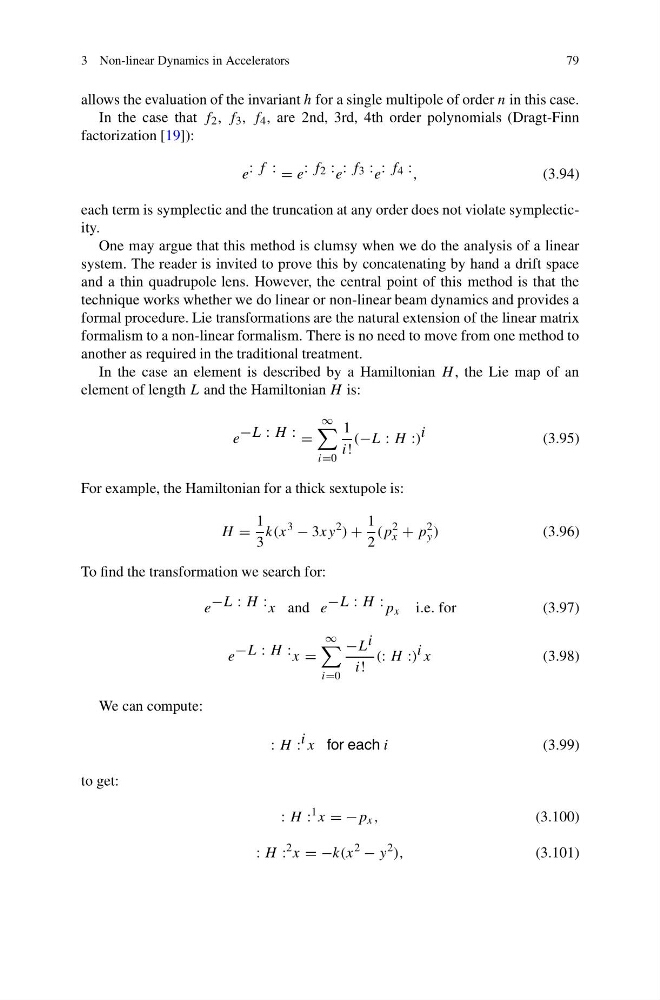
allows the evaluation of the invariant h for a single multipole of order n in this case.
In the case that f 2 , f 3 , f 4 , are 2nd, 3rd, 4th order polynomials (Dragt-Finn
factorization [19]):
e : f : = e : f 2 : e : f 3 : e : f 4 : ,
(3.94)
each term is symplectic and the truncation at any order does not violate symplecticity.
One may argue that this method is clumsy when we do the analysis of a linear
system. The reader is invited to prove this by concatenating by hand a drift space
and a thin quadrupole lens. However, the central point of this method is that the
technique works whether we do linear or non-linear beam dynamics and provides a
formal procedure. Lie transformations are the natural extension of the linear matrix
formalism to a non-linear formalism. There is no need to move from one method to
another as required in the traditional treatment.
In the case an element is described by a Hamiltonian H , the Lie map of an
element of length L and the Hamiltonian H is:
e −L : H : =
∞
i=0
1
i!
(−L : H :) i
(3.95)
For example, the Hamiltonian for a thick sextupole is:
H =
1
3
k(x
3
− 3xy
2 ) +
1
2
(p
2
x + p
2
y )
(3.96)
To find the transformation we search for:
e −L : H : x and e −L : H : p x i.e. for
(3.97)
e −L : H : x =
∞
i=0
−L i
i!
(: H :) i x
(3.98)
We can compute:
: H : i x for each i
(3.99)
to get:
: H :
1 x = −p x ,
(3.100)
: H :
2 x = −k(x
2
− y
2 ),
(3.101)
79
allows the evaluation of the invariant h for a single multipole of order n in this case.
In the case that f 2 , f 3 , f 4 , are 2nd, 3rd, 4th order polynomials (Dragt-Finn
factorization [19]):
e : f : = e : f 2 : e : f 3 : e : f 4 : ,
(3.94)
each term is symplectic and the truncation at any order does not violate symplecticity.
One may argue that this method is clumsy when we do the analysis of a linear
system. The reader is invited to prove this by concatenating by hand a drift space
and a thin quadrupole lens. However, the central point of this method is that the
technique works whether we do linear or non-linear beam dynamics and provides a
formal procedure. Lie transformations are the natural extension of the linear matrix
formalism to a non-linear formalism. There is no need to move from one method to
another as required in the traditional treatment.
In the case an element is described by a Hamiltonian H , the Lie map of an
element of length L and the Hamiltonian H is:
e −L : H : =
∞
i=0
1
i!
(−L : H :) i
(3.95)
For example, the Hamiltonian for a thick sextupole is:
H =
1
3
k(x
3
− 3xy
2 ) +
1
2
(p
2
x + p
2
y )
(3.96)
To find the transformation we search for:
e −L : H : x and e −L : H : p x i.e. for
(3.97)
e −L : H : x =
∞
i=0
−L i
i!
(: H :) i x
(3.98)
We can compute:
: H : i x for each i
(3.99)
to get:
: H :
1 x = −p x ,
(3.100)
: H :
2 x = −k(x
2
− y
2 ),
(3.101)