

78
W. Herr and E. Forest
e : f : [g, h] = [e : f : g, e : f : h]
e : f : (g · h) = e : f : g · e : f : h
and very important:
M g(x) = e : f : g(x) = g(e : f : x)
e.g. e : f : x
2
= (e : f : x)
2
M
−1 g(x) = (e : f : )
−1 g(x) = e − : f : g(x)
note :
1
e : f :
= (e : f : )
−1
(3.89)
3.7.3.2 Concatenation of Lie Transformations
The concatenation is very easy when f and g commute (i.e. [f, g] = [g, f ] = 0)
and we have:
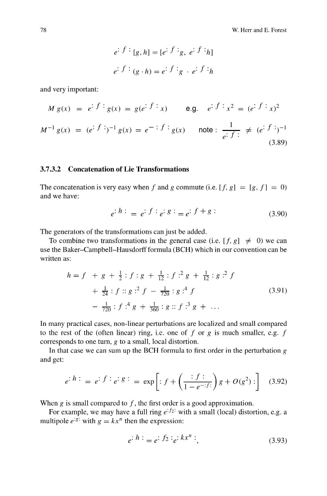
e : h : = e : f : e : g : = e : f + g :
(3.90)
The generators of the transformations can just be added.
To combine two transformations in the general case (i.e. [f, g] = 0) we can
use the Baker–Campbell–Hausdorff formula (BCH) which in our convention can be
written as:
h = f + g +
1
2 : f : g +
1
12 : f : 2 g +
1
12 : g : 2 f
+
1
24 : f :: g : 2 f −
1
720 : g : 4 f
−
1
720 : f : 4 g +
1
360 : g :: f : 3 g + . . .
(3.91)
In many practical cases, non-linear perturbations are localized and small compared
to the rest of the (often linear) ring, i.e. one of f or g is much smaller, e.g. f
corresponds to one turn, g to a small, local distortion.
In that case we can sum up the BCH formula to first order in the perturbation g
and get:
e : h : = e : f : e : g : = exp
: f +
: f :
1 − e −:f :
g + O(g
2 ) :
(3.92)
When g is small compared to f , the first order is a good approximation.
For example, we may have a full ring e :f 2 : with a small (local) distortion, e.g. a
multipole e :g: with g = kx n then the expression:
e : h : = e : f 2 : e : kx n : ,
(3.93)
W. Herr and E. Forest
e : f : [g, h] = [e : f : g, e : f : h]
e : f : (g · h) = e : f : g · e : f : h
and very important:
M g(x) = e : f : g(x) = g(e : f : x)
e.g. e : f : x
2
= (e : f : x)
2
M
−1 g(x) = (e : f : )
−1 g(x) = e − : f : g(x)
note :
1
e : f :
= (e : f : )
−1
(3.89)
3.7.3.2 Concatenation of Lie Transformations
The concatenation is very easy when f and g commute (i.e. [f, g] = [g, f ] = 0)
and we have:
e : h : = e : f : e : g : = e : f + g :
(3.90)
The generators of the transformations can just be added.
To combine two transformations in the general case (i.e. [f, g] = 0) we can
use the Baker–Campbell–Hausdorff formula (BCH) which in our convention can be
written as:
h = f + g +
1
2 : f : g +
1
12 : f : 2 g +
1
12 : g : 2 f
+
1
24 : f :: g : 2 f −
1
720 : g : 4 f
−
1
720 : f : 4 g +
1
360 : g :: f : 3 g + . . .
(3.91)
In many practical cases, non-linear perturbations are localized and small compared
to the rest of the (often linear) ring, i.e. one of f or g is much smaller, e.g. f
corresponds to one turn, g to a small, local distortion.
In that case we can sum up the BCH formula to first order in the perturbation g
and get:
e : h : = e : f : e : g : = exp
: f +
: f :
1 − e −:f :
g + O(g
2 ) :
(3.92)
When g is small compared to f , the first order is a good approximation.
For example, we may have a full ring e :f 2 : with a small (local) distortion, e.g. a
multipole e :g: with g = kx n then the expression:
e : h : = e : f 2 : e : kx n : ,
(3.93)