

48
E. Wilson and B. J. Holzer
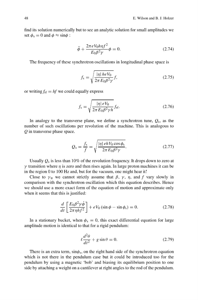
find its solution numerically but to see an analytic solution for small amplitudes we
set φ s = 0 and φ ≈ sinφ :
¨
φ +
2πeV 0 hηf 2
E 0 β 2 γ
φ = 0.
(2.74)
The frequency of these synchrotron oscillations in longitudinal phase space is
f s =
|η| heV 0
2πE 0 β 2 γ
f,
(2.75)
or writing f rf = hf we could equally express
f s =
|η| eV 0
2πE 0 β 2 γ h
f rf .
(2.76)
In analogy to the transverse plane, we define a synchrotron tune, Q s , as the
number of such oscillations per revolution of the machine. This is analogous to
Q in transverse phase space.
Q s =
f s
f
=
|η| ehV 0 cos φ s
2πE 0 β 2 γ
.
(2.77)
Usually Q s is less than 10% of the revolution frequency. It drops down to zero at
γ transition where η is zero and then rises again. In large proton machines it can be
in the region 0 to 100 Hz and, but for the vacuum, one might hear it!
Close to γ tr we cannot strictly assume that β, γ , η, and f vary slowly in
comparison with the synchrotron oscillation which this equation describes. Hence
we should use a more exact form of the equation of motion and approximate only
when it seems that this is justified:
d
dt
E 0 β 2 γ ˙
φ
2πηhf 2
+ eV 0 (sin φ − sin φ s ) = 0.
(2.78)
In a stationary bucket, when φ s = 0, this exact differential equation for large
amplitude motion is identical to that for a rigid pendulum:
d 2 θ
dt 2 + g sin θ = 0.
(2.79)
There is an extra term, sinφ s , on the right hand side of the synchrotron equation
which is not there in the pendulum case but it could be introduced too for the
pendulum by using a magnetic ‘bob’ and biasing its equilibrium position to one
side by attaching a weight on a cantilever at right angles to the rod of the pendulum.
E. Wilson and B. J. Holzer
find its solution numerically but to see an analytic solution for small amplitudes we
set φ s = 0 and φ ≈ sinφ :
¨
φ +
2πeV 0 hηf 2
E 0 β 2 γ
φ = 0.
(2.74)
The frequency of these synchrotron oscillations in longitudinal phase space is
f s =
|η| heV 0
2πE 0 β 2 γ
f,
(2.75)
or writing f rf = hf we could equally express
f s =
|η| eV 0
2πE 0 β 2 γ h
f rf .
(2.76)
In analogy to the transverse plane, we define a synchrotron tune, Q s , as the
number of such oscillations per revolution of the machine. This is analogous to
Q in transverse phase space.
Q s =
f s
f
=
|η| ehV 0 cos φ s
2πE 0 β 2 γ
.
(2.77)
Usually Q s is less than 10% of the revolution frequency. It drops down to zero at
γ transition where η is zero and then rises again. In large proton machines it can be
in the region 0 to 100 Hz and, but for the vacuum, one might hear it!
Close to γ tr we cannot strictly assume that β, γ , η, and f vary slowly in
comparison with the synchrotron oscillation which this equation describes. Hence
we should use a more exact form of the equation of motion and approximate only
when it seems that this is justified:
d
dt
E 0 β 2 γ ˙
φ
2πηhf 2
+ eV 0 (sin φ − sin φ s ) = 0.
(2.78)
In a stationary bucket, when φ s = 0, this exact differential equation for large
amplitude motion is identical to that for a rigid pendulum:
d 2 θ
dt 2 + g sin θ = 0.
(2.79)
There is an extra term, sinφ s , on the right hand side of the synchrotron equation
which is not there in the pendulum case but it could be introduced too for the
pendulum by using a magnetic ‘bob’ and biasing its equilibrium position to one
side by attaching a weight on a cantilever at right angles to the rod of the pendulum.