

9 Accelerator Operations
541
9.5.2.4 Dispersion Measurement
Dispersion is typically inferred from the orbit change induced by a shift in the RF
frequency, see e.g. [13]. This measurement is affected by the BPM calibration errors.
Alternatively it is possible to measure the ratio D x /
√
β x (normalized dispersion)
independently of BPM calibration errors if
√
β x is inferred from the amplitude of
the beam oscillations [48].
9.5.3 Optics Correction Techniques
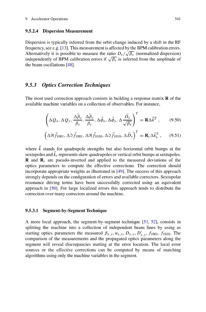
The most used correction approach consists in building a response matrix R of the
available machine variables on a collection of observables. For instance,
x , ,Q y ,
x
β x
,
y
β y
, ,
φ x , ,
φ y , ,
D x
√
β x
T
= R
k
T ,
(9.50)
f 1001 , ,
f 1001 , ,
f 1010 , ,
f 1010 , ,
D y
T = R s
k
T
s ,
(9.51)
where
k stands for quadrupole strengths but also horizontal orbit bumps at the
sextupoles and
k s represents skew quadrupoles or vertical orbit bumps at sextupoles.
R and R s are pseudo-inverted and applied to the measured deviations of the
optics parameters to compute the effective corrections. The correction should
incorporate appropriate weights as illustrated in [49]. The success of this approach
strongly depends on the configuration of errors and available correctors. Sextupolar
resonance driving terms have been successfully corrected using an equivalent
approach in [50]. For large localized errors this approach tends to distribute the
correction over many correctors around the machine.
9.5.3.1 Segment-by-Segment Technique
A more local approach, the segment-by-segment technique [51, 52], consists in
splitting the machine into a collection of independent beam lines by using as
starting optics parameters the measured β x,y , α x,y , D x,y , D
x,y , f 1001 , f 1010 . The
comparison of the measurements and the propagated optics parameters along the
segment will reveal discrepancies starting at the error location. The local error
sources or the effective corrections can be computed by means of matching
algorithms using only the machine variables in the segment.
541
9.5.2.4 Dispersion Measurement
Dispersion is typically inferred from the orbit change induced by a shift in the RF
frequency, see e.g. [13]. This measurement is affected by the BPM calibration errors.
Alternatively it is possible to measure the ratio D x /
√
β x (normalized dispersion)
independently of BPM calibration errors if
√
β x is inferred from the amplitude of
the beam oscillations [48].
9.5.3 Optics Correction Techniques
The most used correction approach consists in building a response matrix R of the
available machine variables on a collection of observables. For instance,
x , ,Q y ,
x
β x
,
y
β y
, ,
φ x , ,
φ y , ,
D x
√
β x
T
= R
k
T ,
(9.50)
f 1001 , ,
f 1001 , ,
f 1010 , ,
f 1010 , ,
D y
T = R s
k
T
s ,
(9.51)
where
k stands for quadrupole strengths but also horizontal orbit bumps at the
sextupoles and
k s represents skew quadrupoles or vertical orbit bumps at sextupoles.
R and R s are pseudo-inverted and applied to the measured deviations of the
optics parameters to compute the effective corrections. The correction should
incorporate appropriate weights as illustrated in [49]. The success of this approach
strongly depends on the configuration of errors and available correctors. Sextupolar
resonance driving terms have been successfully corrected using an equivalent
approach in [50]. For large localized errors this approach tends to distribute the
correction over many correctors around the machine.
9.5.3.1 Segment-by-Segment Technique
A more local approach, the segment-by-segment technique [51, 52], consists in
splitting the machine into a collection of independent beam lines by using as
starting optics parameters the measured β x,y , α x,y , D x,y , D
x,y , f 1001 , f 1010 . The
comparison of the measurements and the propagated optics parameters along the
segment will reveal discrepancies starting at the error location. The local error
sources or the effective corrections can be computed by means of matching
algorithms using only the machine variables in the segment.