

540
M. Lamont et al.
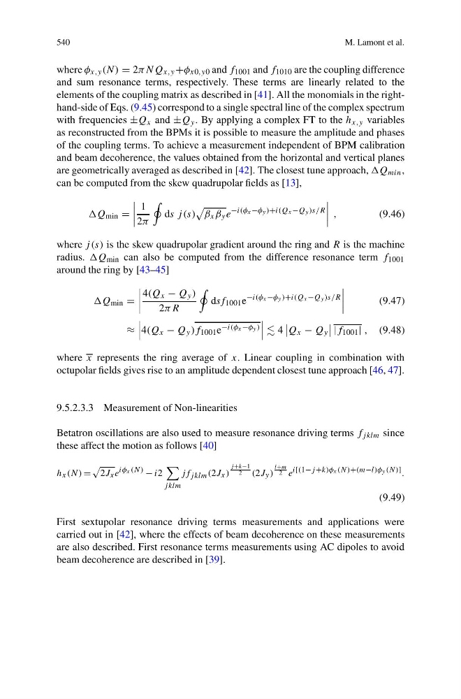
where φ x,y (N) = 2πNQ x,y +φ x0,y0 and f 1001 and f 1010 are the coupling difference
and sum resonance terms, respectively. These terms are linearly related to the
elements of the coupling matrix as described in [41]. All the monomials in the righthand-side of Eqs. (9.45) correspond to a single spectral line of the complex spectrum
with frequencies ±Q x and ±Q y . By applying a complex FT to the h x,y variables
as reconstructed from the BPMs it is possible to measure the amplitude and phases
of the coupling terms. To achieve a measurement independent of BPM calibration
and beam decoherence, the values obtained from the horizontal and vertical planes
are geometrically averaged as described in [42]. The closest tune approach, Q min ,
can be computed from the skew quadrupolar fields as [13],
Q min =
1
2π
ds j (s)
β x β y e
−i(φ x −φ y )+i(Q x −Q y )s/R
,
(9.46)
where j (s) is the skew quadrupolar gradient around the ring and R is the machine
radius. Q min can also be computed from the difference resonance term f 1001
around the ring by [43–45]
Q min =
4(Q x − Q y )
2πR
dsf 1001 e
−i(φ x −φ y )+i(Q x −Q y )s/R
(9.47)
≈
4(Qx − Q y )f 1001 e −i(φ x −φ y )
4
Q x − Q y
|f 1001 | , (9.48)
where x represents the ring average of x. Linear coupling in combination with
octupolar fields gives rise to an amplitude dependent closest tune approach [46, 47].
9.5.2.3.3 Measurement of Non-linearities
Betatron oscillations are also used to measure resonance driving terms f jklm since
these affect the motion as follows [40]
h x (N) =
2J x e iφ x (N) − i2
jklm
jf jklm (2J x )
j+k−1
2
(2J y )
l+m
2 e i[(1−j +k)φ x (N)+(m−l)φ y (N)] .
(9.49)
First sextupolar resonance driving terms measurements and applications were
carried out in [42], where the effects of beam decoherence on these measurements
are also described. First resonance terms measurements using AC dipoles to avoid
beam decoherence are described in [39].
M. Lamont et al.
where φ x,y (N) = 2πNQ x,y +φ x0,y0 and f 1001 and f 1010 are the coupling difference
and sum resonance terms, respectively. These terms are linearly related to the
elements of the coupling matrix as described in [41]. All the monomials in the righthand-side of Eqs. (9.45) correspond to a single spectral line of the complex spectrum
with frequencies ±Q x and ±Q y . By applying a complex FT to the h x,y variables
as reconstructed from the BPMs it is possible to measure the amplitude and phases
of the coupling terms. To achieve a measurement independent of BPM calibration
and beam decoherence, the values obtained from the horizontal and vertical planes
are geometrically averaged as described in [42]. The closest tune approach, Q min ,
can be computed from the skew quadrupolar fields as [13],
Q min =
1
2π
ds j (s)
β x β y e
−i(φ x −φ y )+i(Q x −Q y )s/R
,
(9.46)
where j (s) is the skew quadrupolar gradient around the ring and R is the machine
radius. Q min can also be computed from the difference resonance term f 1001
around the ring by [43–45]
Q min =
4(Q x − Q y )
2πR
dsf 1001 e
−i(φ x −φ y )+i(Q x −Q y )s/R
(9.47)
≈
4(Qx − Q y )f 1001 e −i(φ x −φ y )
4
Q x − Q y
|f 1001 | , (9.48)
where x represents the ring average of x. Linear coupling in combination with
octupolar fields gives rise to an amplitude dependent closest tune approach [46, 47].
9.5.2.3.3 Measurement of Non-linearities
Betatron oscillations are also used to measure resonance driving terms f jklm since
these affect the motion as follows [40]
h x (N) =
2J x e iφ x (N) − i2
jklm
jf jklm (2J x )
j+k−1
2
(2J y )
l+m
2 e i[(1−j +k)φ x (N)+(m−l)φ y (N)] .
(9.49)
First sextupolar resonance driving terms measurements and applications were
carried out in [42], where the effects of beam decoherence on these measurements
are also described. First resonance terms measurements using AC dipoles to avoid
beam decoherence are described in [39].